It is often the case that you will need to use functions as arguments within other functions, in order to achieve your objectives
When a function is used as an argument in another function, it is referred to as a "nested" function
In this lecture, we will go over some simple examples to help acclimate you to nested functions
We will also go through a comprehensive, practical example demonstrating the use of nested functions
In this example, we will also provide you with a technique which can help you build complex formulas more easily
Examples
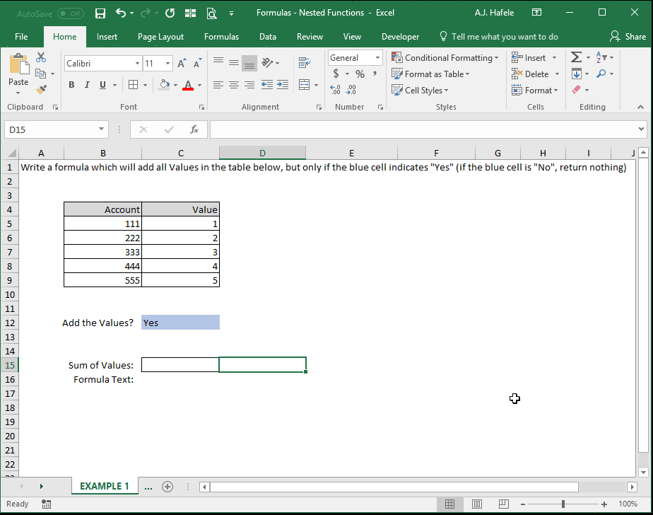
Observe as we use the SUM function nested in the IF function to add numbers only if a certain condition is met:
Here is a screenshot, for reference:
This one is pretty straightforward - a SUM calculation will be made only if the blue cell is "Yes"
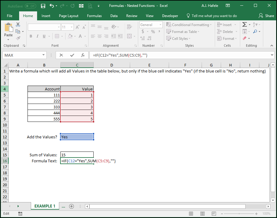
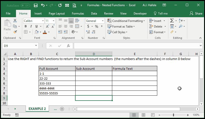
Next, observe as we use the RIGHT and FIND functions to return an idiosyncratic set of sub-account numbers:
Here is a screenshot, for reference:
What is going on here?
First, we know we need to return the right x-most digits of the Full Account numbers
But "x" is not constant, since the Full Account numbers are idiosyncratic in length
To resolve this, we simply use FIND to return the numerical position of the dash in each row
We subtract 1 because we do not want to include the dash the Sub Account number in column D
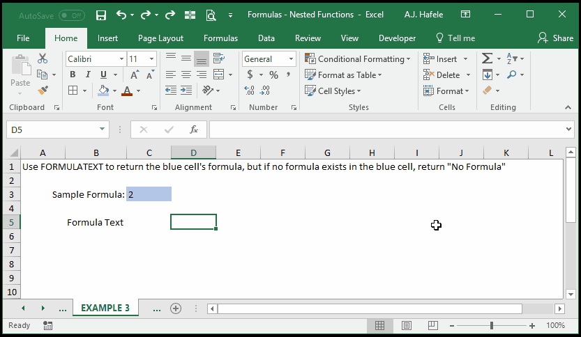
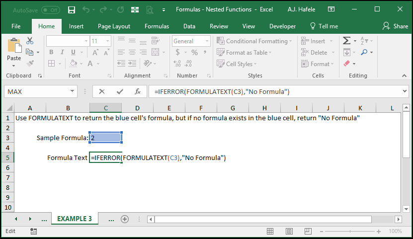
Last, let's wrap the FORMULATEXT function around the IFERROR function to remove those ugly errors when no formula exists:
This one should look familiar, as we have used the technique throughout the course in our illustrations!
Here is a screenshot, for reference:
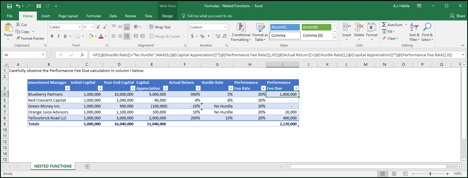
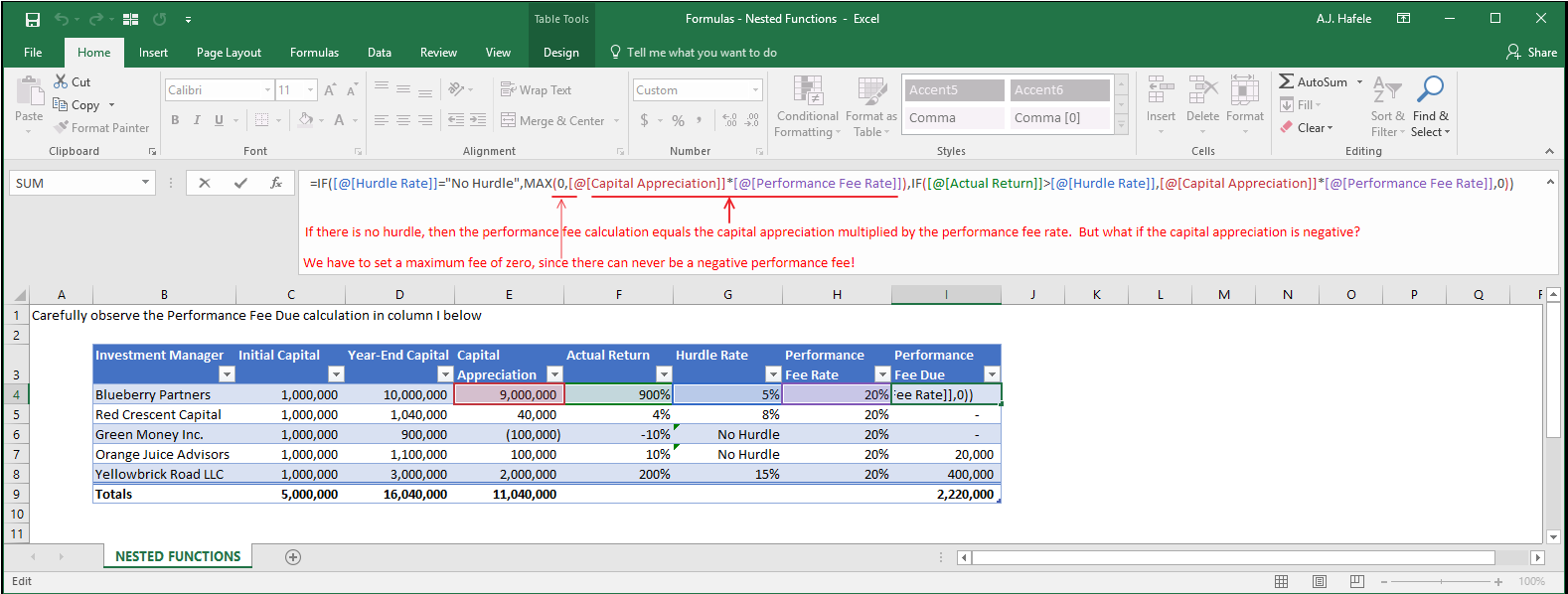
Practical Example - Investment Performance Fee Calculation
Imagine you have hired 5 investment managers to invest $5 million on your behalf
You have 5 separate agreements to pay out a performance fee to the managers at the end of the year
The performance fee due is calculated by multiplying a performance fee rate by the capital appreciation for the year
For example, if a manager's capital appreciation is $1,000,000 in one year, and the performance fee rate is 20%, that manager gets a $200,000 performance fee
However, a performance fee is only earned under certain conditions:
First, the manager must have had a positive return (i.e. the manager actually made you money) in order to receive a performance fee payment
Second, in certain (but not all) arrangements, the manager's annual return must exceed a hurdle rate
Think of a hurdle rate as a threshold return percentage that must be met in order for a manager to earn any performance fee
For example, if the manager makes a +5% return, but the hurdle rate is +6%, that manager gets $0 in performance fees!
On the other hand, if the manager made a +7% return, a performance fee is earned on the full capital appreciation
In our example below, 3 of the 5 managers must surpass a hurdle rate, but 2 will not
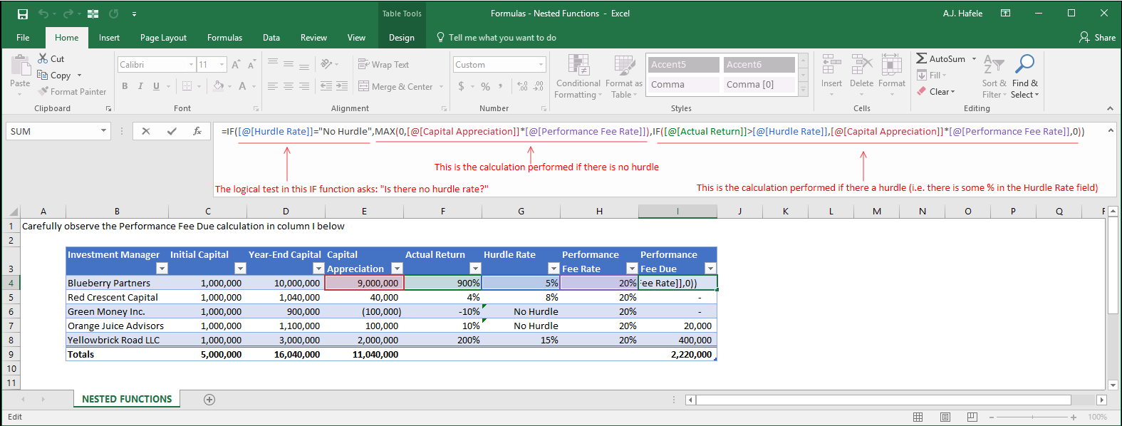
Here is a screenshot of our worksheet with our performance fee calculations for each manager (focus on the formula in column I, which can be seen in the formula bar):
(Blueberry clearly dominates, but that is beside the point)
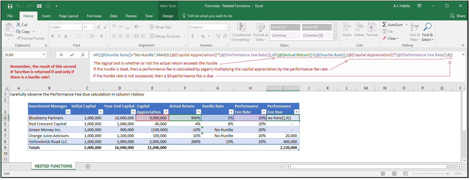
Let's analyze this function in more detail, starting with the outer (primary) IF function:
Notice that the latter 2 arguments of the IF function above have nested functions:
The value_if_true argument has a MAX function
The value_if_false argument has another IF function
Let's now look at the MAX function in the value_if_true argument:
Last, let's look at the value_if_false argument (which contains another IF function):
Notice that this IF function also accommodates for negative returns nicely, since the hurdle rate is always positive
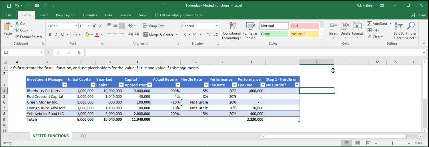
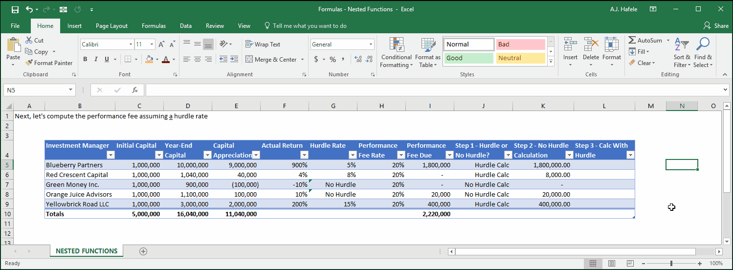
Now, let's walk through an easy and systematic way to create this (large) formula
Practical Example - Technique For Building Complex Formulas
To demonstrate, we will continue with the performance fee calculation above
Step 1: We will start by creating the outermost IF function, which asks if there is a hurdle rate or not
Instead of adding the two nested functions, let's keep it simple and just leave some temporary placeholders, as shown here:
The placeholders - "No Hurdle Calc" and "Hurdle Calc" - will be substituted later with the appropriate calculations
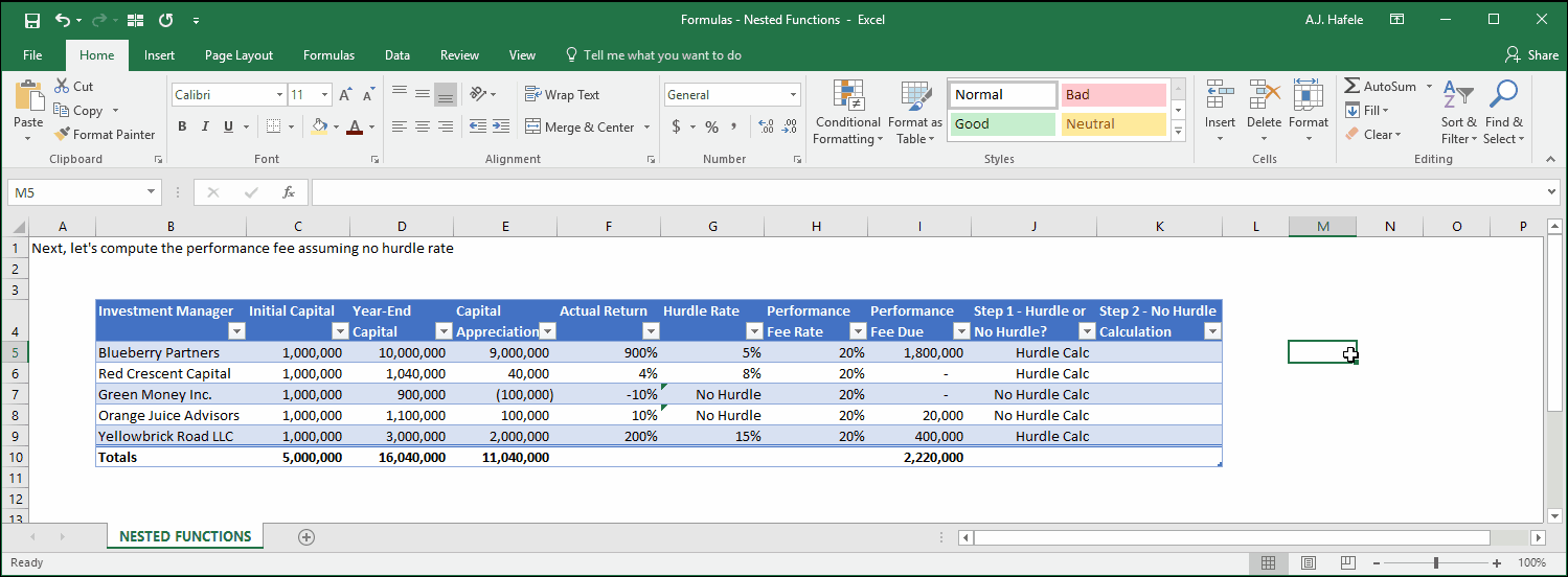
Step 2: Let's perform (in a separate column) the fee calculation assuming no hurdle rate, as shown here:
Step 3: Let's perform (in a separate column) the fee calculation assuming a hurdle rate, as shown here:
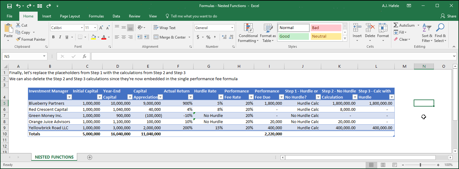
Step 4: Let's replace the placeholders in the IF function created in Step 1 with the functions created in Step 2 and Step 3 (avoid copying and pasting the = signs):
Note that the results in column J now match those of column I
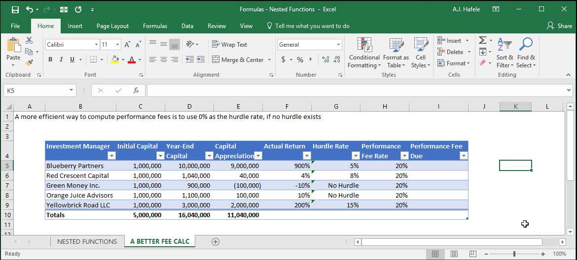
Practical Example - A More Efficient Fee Calculation Method
You may have recognized that the huge calculation above can actually be avoided!
How? Instead of hard-coding "No Hurdle" in the Hurdle Rate field, enter 0% instead, since that is effectively the same as no hurdle
This is also desirable because you should avoid mixing text (e.g. "No Hurdle") with numerical data (e.g. "5%")
Observe that we get the same results with a more simple formula (a single IF function, which is the same as the one in Step 3 above):
Final Comments
As the final example shows, you can very quickly build very large formulas with lots of nested functions
But remember that these larger formulas are ultimately built from the much more simple functions and calculations!