Array formulas are used to perform calculations which typically cannot be performed with the standard Excel functions alone
They are also used to to reduce or eliminate intermediate calculations which would have been otherwise necessary
They are referred to as "array formulas" because arrays (or ranges) of cells or constants are used somewhere within the formulas, typically in ways that are not intuitive at a first glance
Here are some examples of array formulas:
{=A1:A10+5}
{=SUM(A1:A10/B1:B10)}
Upon close inspection, these do not seem very intuitive, but they will become more clear as we go though some examples
There are two types of array formulas that can be created
Multi-cell array formulas: array formula results will be stored in multiple cells
Single-cell array formulas: array formula results will be stored in a single cell
Also, as a consequence of learning about array formulas, we will review how to use the MODE.MULT and TRANSPOSE formulas
Creating Array Formulas
Before we jump into examples, let's quickly review how array formulas are created
At this point, you know that pressing ENTER after writing a formula will store the formula into a cell
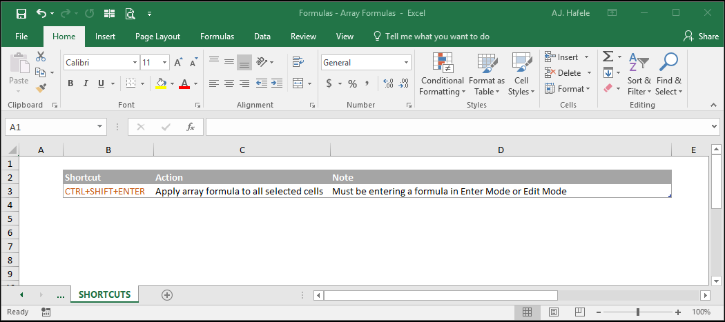
To create an array formula (either multi-cell or single-cell ones), you must press CTRL+SHIFT+ENTER after writing the formula, rather than just ENTER alone
Upon pressing CTRL+SHIFT+ENTER, braces (also referred to as curly brackets) are placed at the beginning and end of the array formulas
Now that you know how to create array formulas, let's go through some illustrations
Multi-Cell Array Formulas
As mentioned above, multi-cell array formulas will place formula results in multiple cells, rather than within a single cell
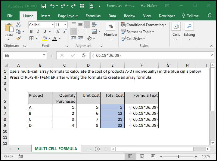
Observe as we write one array formula to calculate the cost of four products (in 4 different cells), using the CTRL+SHIFT+ENTER shortcut:
Here is a screenshot, for reference:
Notice that:
Before writing the array formula, we selected all four blue cells
We entered a single formula in cell E6 and then pressed CTRL+SHIFT+ENTER to store the array formula
All four cells containing the array formula contain the exact same formula
The presence of an array formula is evidenced by the braces around the formulas
If you need to delete a multi-cell array formula, you must select and delete the entire array, as shown here:
In this illustration, all 4 blue cells had to be selected in order to delete the array formula
Why Use Multi-Cell Array Formulas?
In the above example, we did not need to use a multi-cell array formula
We simply could have used =C6*D6 in cell E6, and copied and pasted that formula down
So why ever use array formulas?
Microsoft tell us (per the links below) that the advantages are:
Greater consistency, since a single formula is used
Safety, since you cannot accidentally delete one part of an array formula
Smaller file size (since one formula is used instead of multiple)
In addition, multi-cell array formulas can help you understand how to use single-cell array formulas (which have many more interesting uses)
It is also worth mentioning that some new Excel functions were created to work with multi-cell array formulas
To illustrate, the MODE function is limited in Excel, since only one mode can ever be presented
However, Microsoft created the MODE.MULT function, which can be used in multi-cell array formulas to capture multiple modes instead, as shown here:
Notice that:
Since we wanted to find at least 3 modes, we had to select 3 cells before writing our array formula
Upon deleting one instance of the number 1, it is no longer a mode, and so the MODE.MULT result is updated to contain 2, 3, and #N/A (since there are only two modes now)
The disadvantage of array formulas, however, is that they are not commonly used, and as such, users may have trouble working with them
Generally speaking, we would recommend that you avoid using multi-cell array formulas, unless they are necessary
Single-Cell Array Formulas
In contrast to multi-cell array formulas, single-cell array formulas are stored in just one cell (as you should be comfortable with by now)
Of course, you still press CTRL+SHIFT+ENTER to create single-cell array formulas
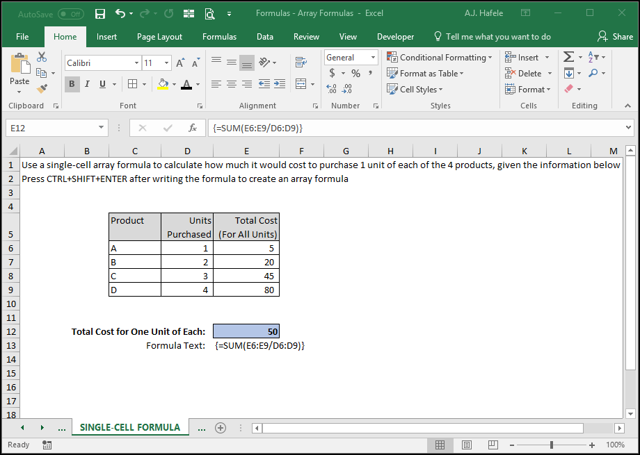
In the following illustration, we use a single-cell array formula to compute the cost of purchasing one of each of 4 products, given a certain set of information:
Here is a screenshot, for reference:
How does this formula work?
Excel is taking corresponding elements in each array (e.g. E6 and D6), dividing them to get 4 results, and then adding the 4 results
In other words, the formula is exactly the same as =SUM(E6/D6,E7/D7,E8/D8,E9/D9), but it is much easier to write, and it can accommodate for row insertions and/or deletions
Note that we could have divided column E by column D in column F (and then added), but if the individual per-product cost information were not relevant, the single-cell array formula will allow you to skip that intermediary task completely
This single-cell array formula is actually a lot like SUMPRODUCT, but with division instead
However, since there is no such thing as a SUMQUOTIENT function, this array formula will suffice
Likewise, SUMAVERAGE, PRODUCTSUM, AVERAGEPRODUCT, and PRODUCTAVERAGE functions do not exist, but you could create single-cell array formulas to accomplish the same objectives
Arrays of Constants (Hard-Coded Numbers)
It is also worth noting that you can indeed enter arrays of constants in cells
Observe as we enter the constants 1 through 4 in both horizontal and vertical ranges of cells:
Notice that:
You must wrap your constants in braces
You must use commas for horizontal arrays of constants
You must use semicolons for vertical arrays of constants
You must still press CTRL+SHIFT+ENTER to store your array of constants (and braces will be wrapped around your entire formula)
You can also use arrays of constants in single-cell array formulas, as shown here:
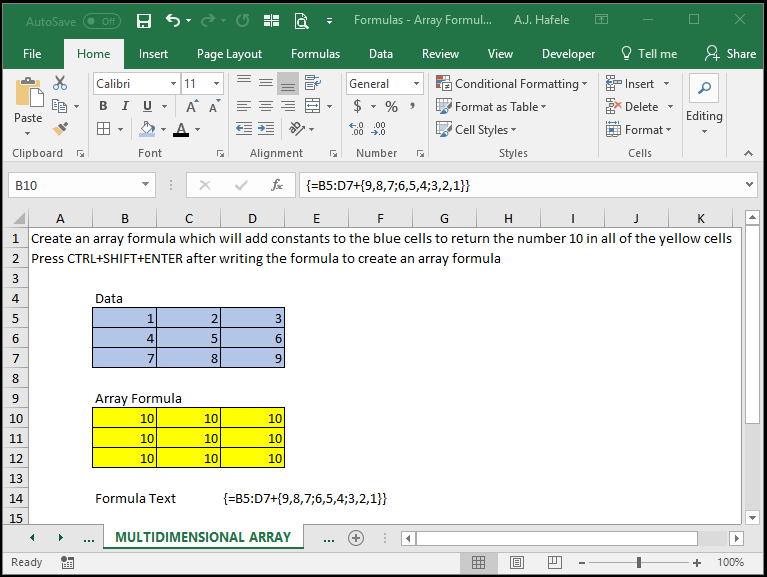
Moreover, using the same rules for constants described above, you can also create multidimensional arrays, as shown here:
Here is a screenshot, for reference (pay close attention to the placement of the commas and semicolons):
In this illustration, the blue cells are multiplied by a 3-by-3 array of constants
In other words, this formula is effectively the same as writing =B5+9 in cell B10, =C5+8 in cell C10, etc.
While not meaningful on their own, these illustrations help show you how Excel is designed to handle arrays of constants
Transposing Arrays
It is important to note that, when using more than one array in an array formula (multi-cell or single-cell), all of the arrays must be of the exact same dimensions
For example, within an array formula, you cannot multiply an array that is 10 rows and 2 columns by an array that is 2 rows and 10 columns, even though both arrays consist of exactly 20 cells
However, you can use the TRANSPOSE function to effectively "flip" an array on its side, such that Excel reads it as having the same dimensions
Continuing with the example mentioned above, you can flip the second array so that Excel treats it like it has 10 rows and 2 columns (even though it actually has 10 columns and 2 rows)
Conceptually, when Excel converts cell ranges to array constants upon performing calculations, the TRANSPOSE function will swap commas for semicolons, and semicolons for commas
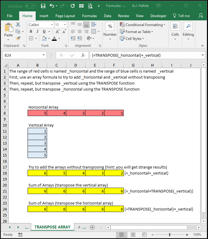
The following illustration highlights these facts (the goal of the illustration is to add two arrays so that each cell in a multi-cell array formula returns the number 6):
Here is a screenshot, for reference:
Notice that:
Without transposing, the number 1 (the topmost value in the _vertical array) is added to the _horizontal range, which is not what we wanted
Upon transposing one of the arrays, the arrays' dimensions become the same (either 5 columns and 1 row, or 1 column and 5 rows), which allows us to successfully return the number 6 in each cell
This illustrates the fact that you should ensure that all arrays are of the same dimensions when performing calculations (and you should take advantage of the TRANSPOSE function if possible)
Final Example
Let's move on to one last challenging example!
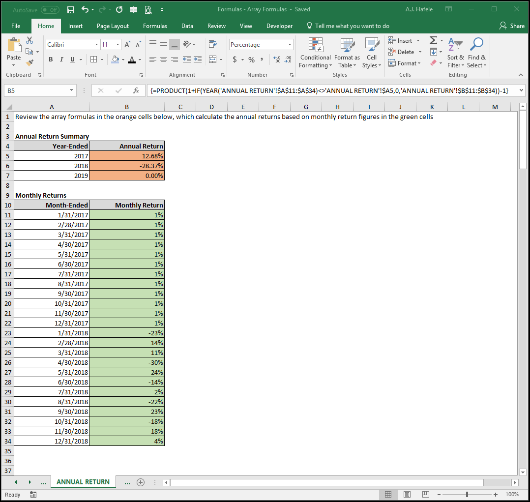
Observe the array formula (containing nested functions) in the following screenshot, which is used to calculate annual returns (think: stock market returns) based on monthly return data for the relevant calendar year:
Note that the same formula has been copied down to cells B6 and B7
A 0% return in 2019 is due to the fact that there are no monthly 2019 return data
What is the array formula actually calculating in the orange cells? Let's break it down:
Step 1: It adds 1 to each monthly return whose month-ended year matches the year-ended (in the top table)
Note that if the monthly return is not in the year in question, it adds 0 to the number 1
For example, for 2017, any month whose year is not 2017 will return the number 1 (since zero is added to it)
Step 2: The product of all numbers calculated from the first step above is computed
E.g. for 2017, the calculation is 1.01 x 1.01 x 1.01 x 1.01 x 1.01 x 1.01 x 1.01 x 1.01 x 1.01 x 1.01 x 1.01 x 1.01 x 1 x 1 x 1 x 1 (and so on)
Step 3: 1 is subtracted from the second calculation described above
E.g. 1.1267 - 1 = .1268 or 12.68%
The beauty of this array formula is that you do not need to bother creating any messy intermediary formulas to obtain annual returns!
.gif)