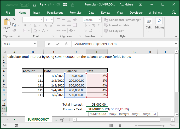
First calculates the product of a set of ranges, and then adds the resulting products
The visualization makes it easier to understand
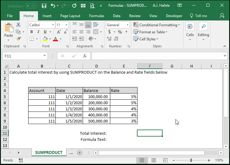
Example
Here is a screenshot for reference:
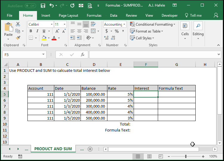
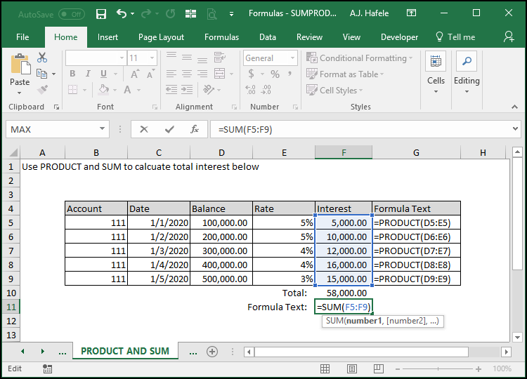
To show you how SUMPRODUCT works, let's instead calculate interest by using the PRODUCT and SUM functions:
Here is a screenshot for reference:
As this example indicates, the products of corresponding cells are first calculated, and then the resulting products are added together to get the final output
Syntax
=SUMPRODUCT(array1, array2, etc.)
Arguments
array1
This is the first range of numbers, which is typically a range of cells
Note that all future arrays in the function must contain the same count of cells as array1
In other words, if array1 is a range of 10 cells, all future arrays must have exactly 10 cells as well
Also, if array1 is horizontal, all future arrays must be horizontal (but not necessarily adjacent to array1)
See the screenshot in the Tips section below for an example
array2
This is the second range of data which will be multiplied by the first range (and all future ranges). For example:
The topmost cell in array1 will be multiplied by the topmost cell in array2 [optional]
The second cell in array1 will be multiplied by the second cell in array2
Etc.
This argument has the same properties as array1
Again, if array1 encompasses 10 cells, array2 must also encompass 10 cells
Again, if array1 is a horizontal range, array2 must also be a horizontal range
The pattern continues (up to 255 arrays for later versions of Excel)
All future arguments have the same properties as array1
Again, all arrays must contain the exact same dimensions (e.g. 10 cells), and all ranges must be either vertical or horizontal
Tips
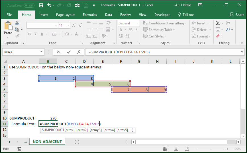
As mentioned above, SUMPRODUCT works for horizontal arrays, as well as non-adjacent arrays, as shown here:
Notice that:
Each array has (and must) contain the same number of cells (3 in this case)
270 is computed by computing the sum of the products of array1, array2, and array3