This is the first value or range of values that you want to add
This can be a hard-coded number (e.g. 100), (single or multiple) cell range (e.g. A1, or A1:A100), or calculation (e.g. A1*200/B1)
number2 [optional]
This is the next number or range in the series
This argument has the same properties as number1
The pattern continues (up to 255 numbers for later versions of Excel)
All remaining arguments have the same properties as number1
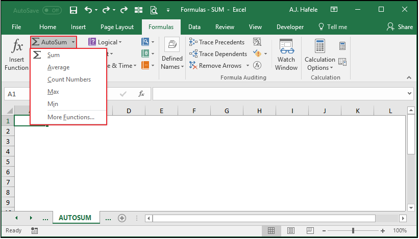
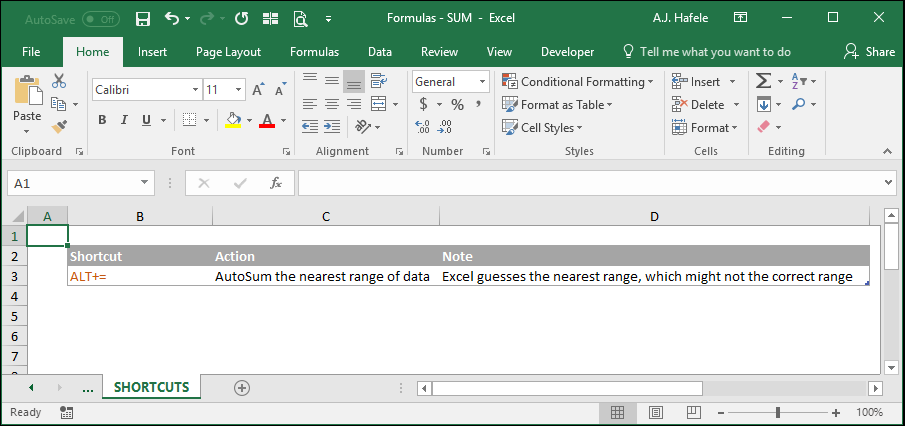
AutoSum
AutoSum is a very handy tool to perform fast SUM calculations
To use AutoSum, place the active cell near the closest contiguous range of numbers and press the AutoSum button (or press ALT+=), as shown here:
Notice that:
AutoSum works for vertical or horizontal ranges (it automatically guesses whether to sum vertically or horizontally)
Again, AutoSum works for contiguous ranges only (i.e. a list of numbers not separated by a blank cell or cell containing text)
Observe what happens if AutoSum is used on non-contiguous range:
Notice that:
AutoSum could not capture the top numbers to add, due to the blank cell and the cell containing text
We had to manually select the entire range to capture all applicable cells
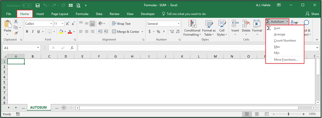
Excel also enables you to perform AutoSum-like calculations with the following buttons (located in the Function Library group of the Formulas tab):
For example selecting "Average" from this drop-down will perform an auto-average of the nearest contiguous range
It is worth mentioning that the AutoSum button can also be found on the Editing group of the Home tab:
Tips
Avoid hard-coding numbers as much as possible
For example, =SUM(1.4444,1.04248,1.20449) can get very messy, especially if the SUM function must get updated frequently
Instead, put individual numbers in their own cells, and reference those cells in the SUM function
This tip applies to more than just the SUM function
When adding a new value to the end of a row or column to be summed, ensure SUM captures the newly-added value
How? Use a blank "buffer" cell at the end of your sum range, as shown here:
If you do not include a buffer, your SUM formula will not automatically adjust to capture newly-inserted data, as shown here:
This tip is also applicable to more than just the SUM function
As a better alternative to using a buffer, simply insert and use a table (no need to skip ahead, however)
The SUM function is generally superior to using the "+" operator. Why? Using =A1+B1+C1 as an example:
What if A1 contained text, such as "Hello"?
You will get a #VALUE! error
You will not get this error if you used =SUM(A1:C1)
What if you needed to insert a new column between columns A and B (which also needed to be added)?
=A1+B1+C1 would turn into =A1+C1+D1, but the new B1 is missing
The SUM function would adjust to be =SUM(A1:D1)
What if you deleted column B completely?
=A1+B1+C1 would turn into =A1+#REF+C1, which translates into =#REF
The SUM function would adjust to be =SUM(A1:B1)
See a similar example (of deleting a row) in the following illustration:
Last, we have not yet discussed how to group and hide rows and columns (no need to skip ahead), but you should be aware of the following at this point:
You can hide rows and columns from view
Certain functions, including SUM, will still reference hidden cells when performing calculations, as shown here:
As you can see, the SUM result is still 5, despite the fact that two numbers were hidden
Note that there are some functions - namely SUBTOTAL - which can exclude hidden cells when performing calculations