Looks up a user-defined value contained in a single column or row of data, and returns the relative numerical position of that value within the range
If no match is found, #N/A is returned
Examples
The first example illustrates how to find the relative row number of a single column of data:
Here is a screenshot, for reference:
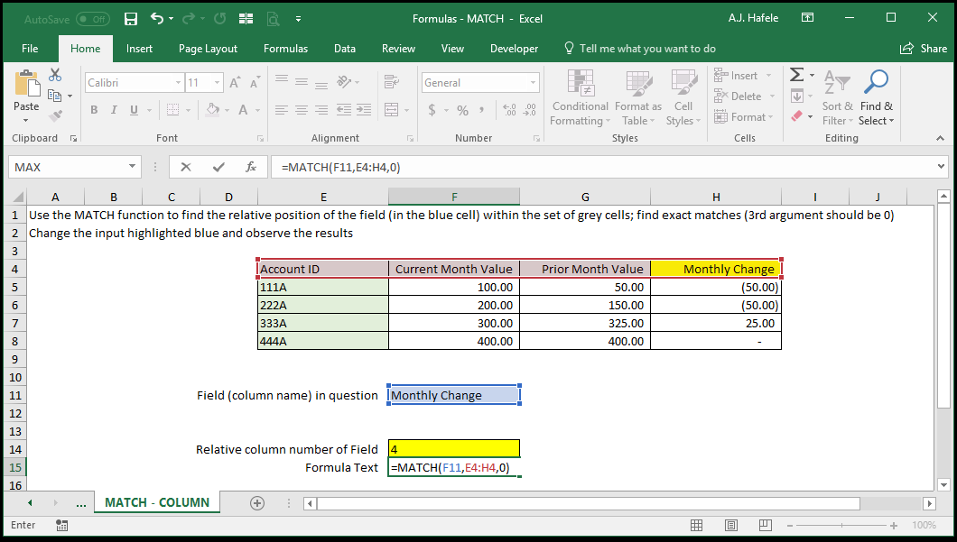
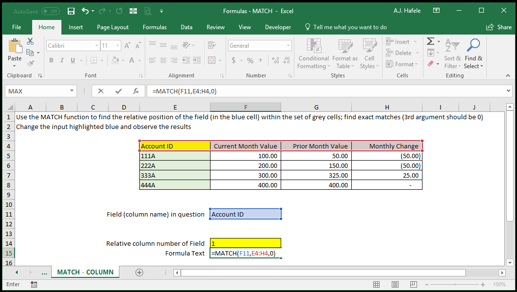
The second example illustrates how to find the relative column number of a single row of data:
Here is a screenshot, for reference:
Note that an error will occur if the second argument is a range covering multiple rows and columns (again, the range should be a single row or column of data)
Syntax
=MATCH(lookup_value, lookup_array, match_type)
Arguments
lookup_value
This is the value that you need the relative cell position for (within the lookup_array)
This value is case-insensitive
This can be a hard-coded value (text or number), cell reference, or calculation
lookup_array
This is a contiguous range of cells which should contain the lookup_value
This should be a single-row or single-column range only (if not, you will get an error)
match_type [optional]
Can be one of the following:
-1: Finds the smallest value that is greater than or equal to the lookup_value
The lookup_array must be in descending order
0: Finds the first value that is exactly equal to the lookup_value
The lookup_array can be in any order, but remember that the position of the first instance of the lookup_value found will be returned
This value requires the most precision (an exact match must be in the lookup_array)
1 (or omitted): Finds the largest value that is less than or equal to the lookup_value
The lookup_array must be in ascending order
This can be a hard-coded number, cell reference, or calculation
Tips
The MATCH function is often used with the INDEX function to return a data point within a table of data