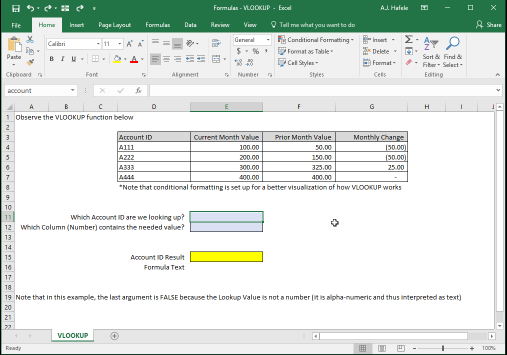
Looks up a user-defined value in the leftmost column of a range of data, and provides a corresponding data point in a user-defined column within that same range of data
Example
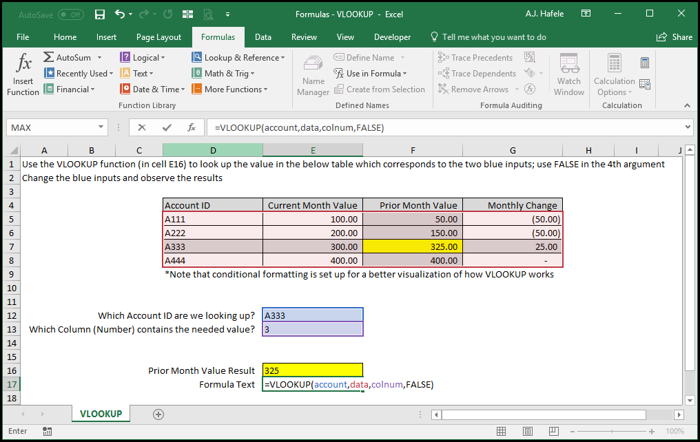
In this example, we use the following 3 named ranges:
"account" (cell E12)
"colnum" (cell E13)
"data" (cells D5:G8)
Additionally, we added conditional formatting in the "data" range to show you exactly which value is being looked up (the highlighted figure)
Here is a screenshot, for reference:
Notice that:
The value in the 3rd column (Prior Month Value) in the row corresponding to A333 is 325 (the two highlighted figures)
When we change one of the two blue inputs, a new number is looked up
Essentially, VLOOKUP finds the value in your table of data (2nd argument) that is at the intersection of:
The row corresponding to the 1st argument (account)
The column number you provide in the 3rd argument (colnum)
This is the value that you would like to look up in your table_array
This can be a hard-coded value (text or number), cell reference, or calculation
table_array
This is a contiguous range of cells
The leftmost column should always contain the data corresponding to the lookup_value
col_index_num
This is the column number of the table_array range selected which contains the desired resulting value
Note that the leftmost column in the table_array is column 1
This can be a hard-coded number, cell reference, or calculation
range_lookup [optional]
Only omit this value (or enter TRUE, or 1) when the lookup_value is numerical and you are okay with finding a resulting value approximately corresponding to your lookup_value
If omitted, TRUE, or 1, Excel will find the value closest to the lookup_value (by always rounding down to the nearest lookup_value) in the table_array and return the resulting value that is located in the col_index_num
If you need to omit or use TRUE for this argument, the data must be sorted in ascending order (e.g. 1 to 10)
If FALSE or 0, Excel will only return the value in the col_index_num if the leftmost column contains the exact lookup_value
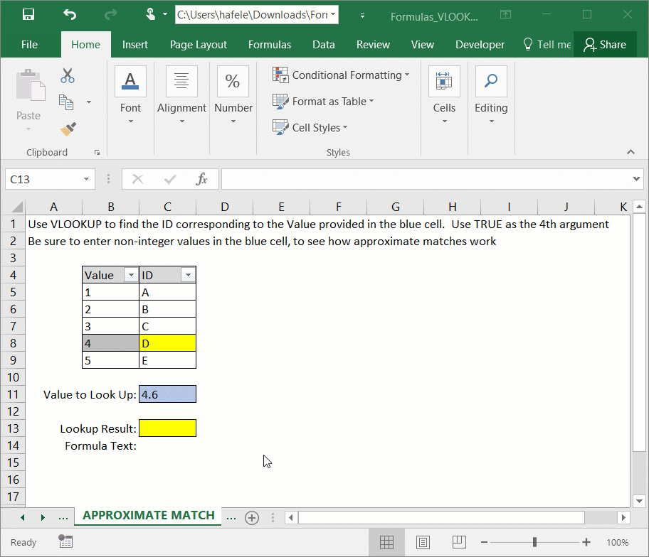
Approximate Matches (4th Argument is TRUE)
What if we need to get approximate matches when looking up numerical values? How does VLOOKUP work?
As mentioned above, VLOOKUP will essentially round the lookup_value down to the closest lookup value, as shown here:
Here is a screenshot, for reference:
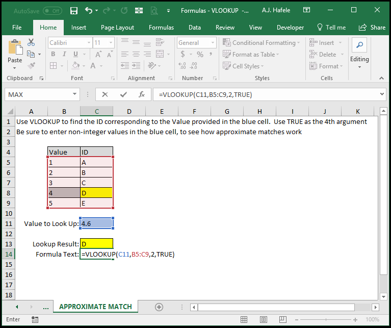
Note that:
Regardless of the decimal, all numbers are rounded down
In the above example, the closest match to 4.6 when rounding down is 4
If the number 4 were not in the table_array at all, 4.6 would then round down to 3
If the lookup_value entered is lower than the lowest value in the table_array, the #N/A error is returned
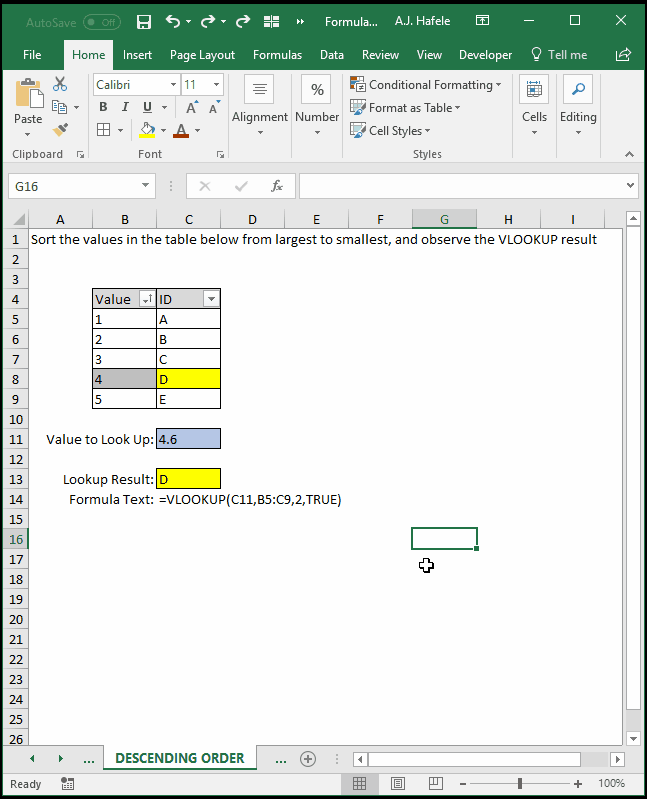
Again, if you are using VLOOKUP with approximate matches, you need to be sure the leftmost data in the table_array is sorted from smallest to largest
Observe what happens if you do not do this:
As you can see, the VLOOKUP result changed to A, which makes no sense in this context!
Tips
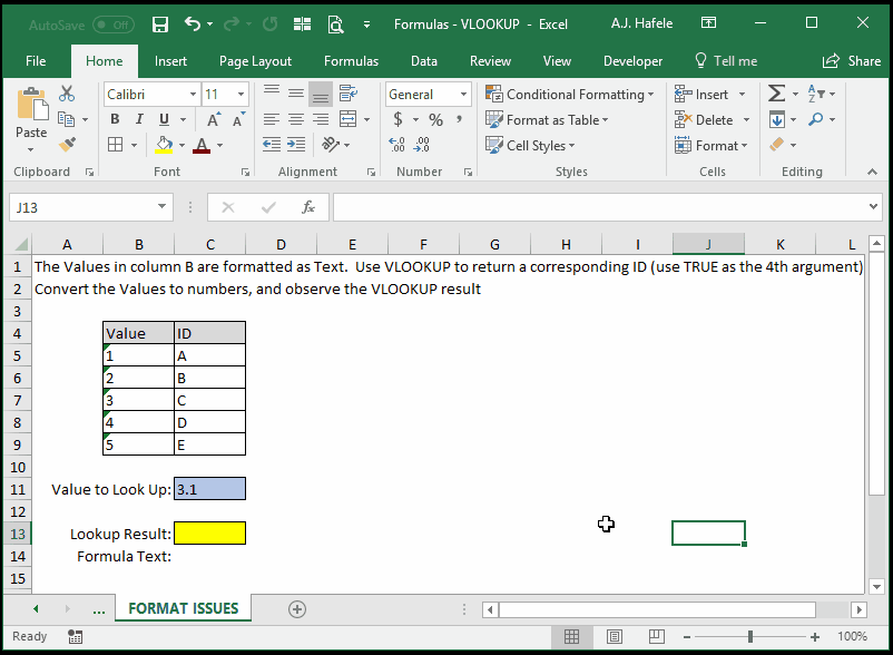
As per the Number and Text Formats lecture, you should recognize that numbers formatted as Text may not be properly referenced using VLOOKUP when the lookup_value is formatted as a number, but the leftmost column in the table_array contains data formatted as Text, or vice versa
The following illustrates what happens when this occurs:
Notice that:
The #N/A error initially occurred because the lookup_value was interpreted by Excel as a number, but the Values in the table_array were formatted as Text
Once the Values in the table_array were converted to numbers (consistent with the format of the lookup_value), the error went away
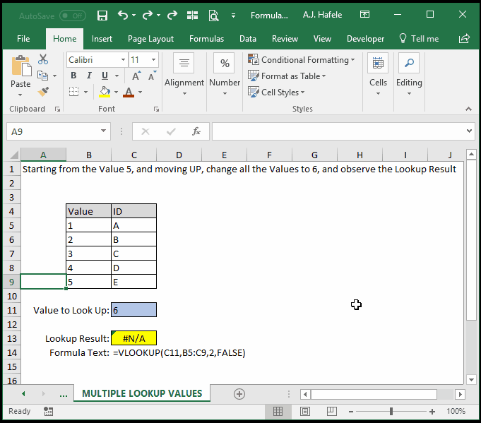
Last, be careful when the lookup_value is found multiple times in the table_array, as shown here:
As you can see, when we are trying to get an exact match (range_lookup is FALSE), the topmost row containing the number 6 is used to return the output
This may not be desirable, and as such, VLOOKUP may not be useful in such situations