Filtering is another essential functionality in Excel
Filtering allows you to hide rows of data that you do not care to look at, temporarily (the data are not deleted)
You can filter multiple fields if desired
As with sorting, filtering can be performed on ranges of cells, or within tables
Buttons
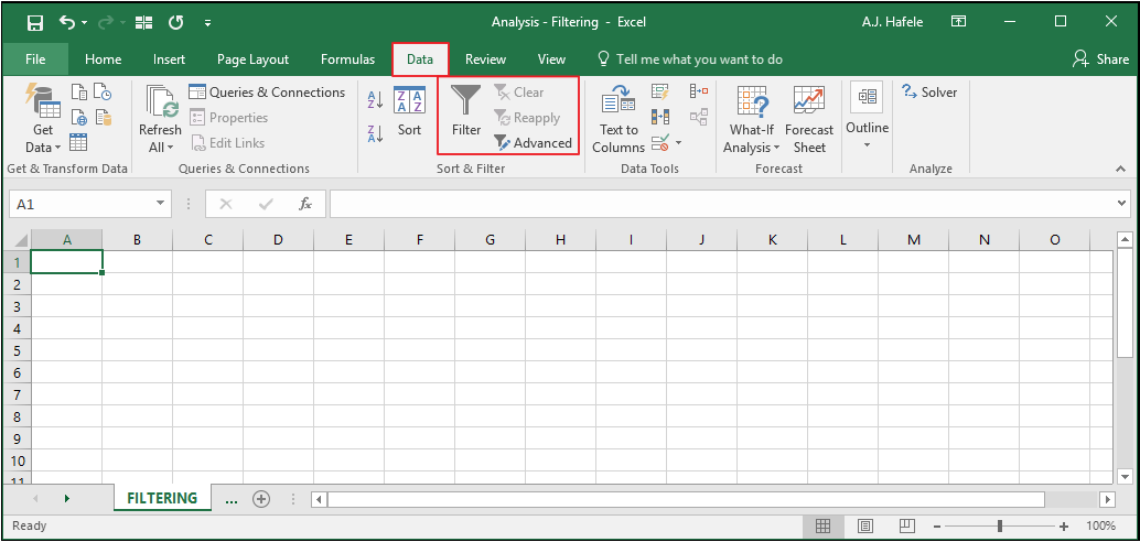
The relevant buttons can be found in the Sort & Filter group of the Data tab:
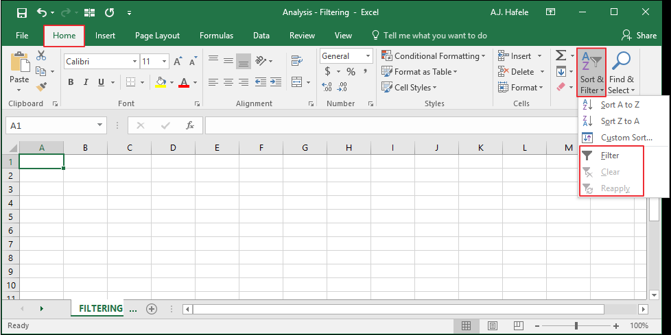
You can also find the same buttons in the Editing group of the Home tab:
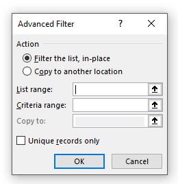
The following menu appears when clicking the Advanced (Filter) button in the Data tab:
We will discuss advanced filtering at the end of this lecture
Examples
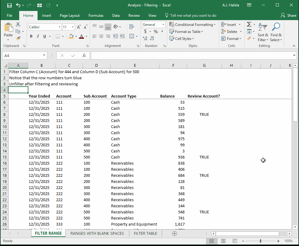
In the first illustration, let's filter a single field in a range of data
Note that we will first add filter buttons in order to filter the data:
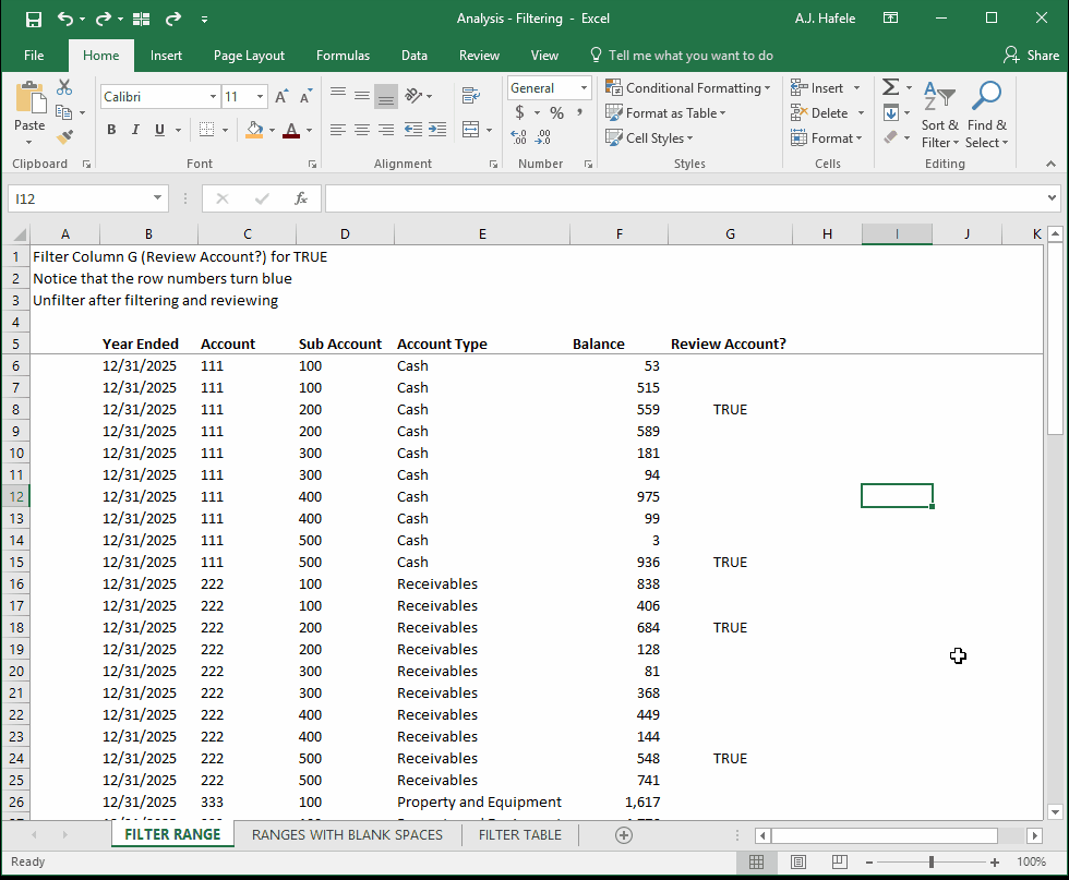
Remember to keep an eye out on the row numbers on the left-hand side - blue row numbers mean that the rows are filtered!
Now, let's filter 2 fields in the range this time, using the Filter button in the Data tab:
Notice in both examples above that Excel automatically determined the range of cells that was captured in the filter (B65:G65)
Although this automatic determination is convenient, we highly recommend selecting the entire range manually. Why? To ensure the entire range is selected (and subsequently filtered)
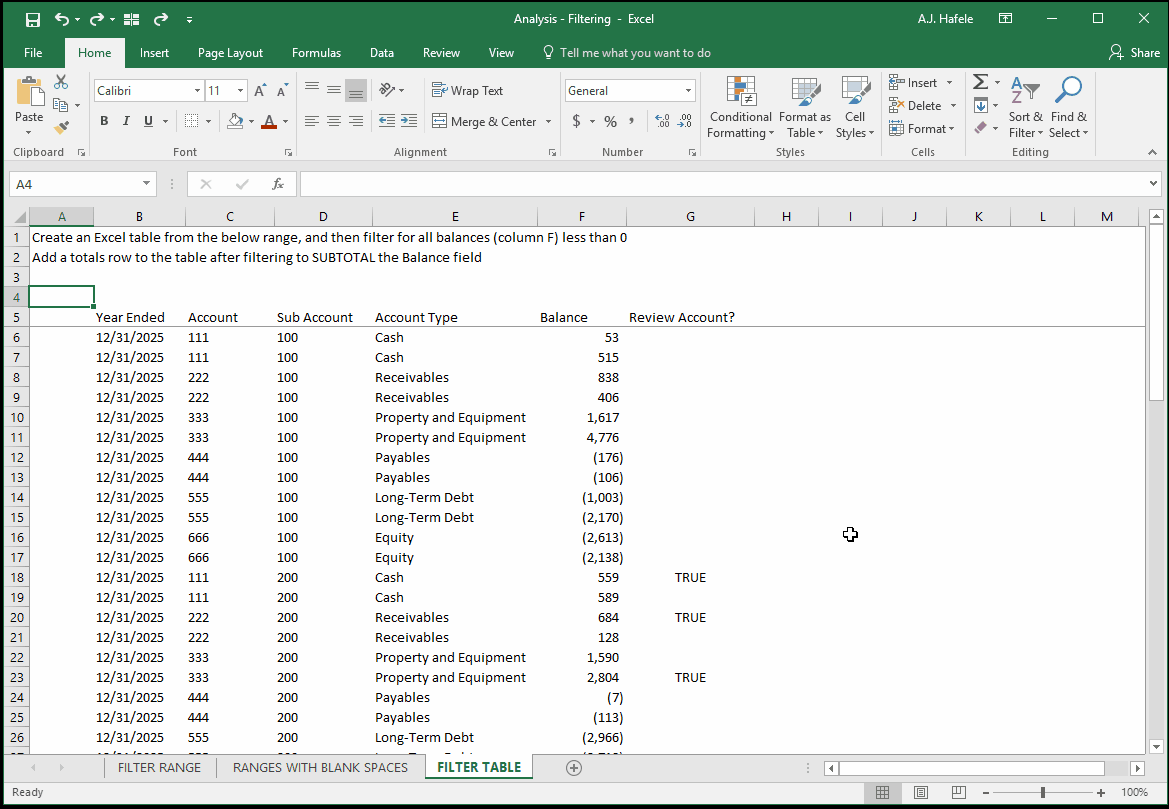
Better yet, if put your data in a table, you won't need to worry about not capturing all the data!
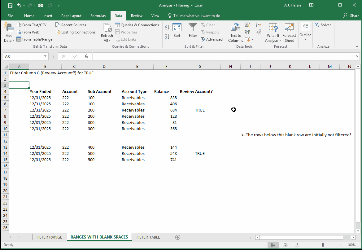
In the next illustration, notice that the bottom 3 rows are missed on the initial filter, but subsequently filtered the second time around, after selecting the entire range:
Remember, as an alternative to clicking the filter buttons as shown above, you can use the CTRL+SHIFT+L shortcut
Again, however, you should ensure that the entire range of data is captured
Also, remember that if you data were in a table, however, the filter buttons, once toggled on, will always capture the entire range!
Let's now create a table (which will automatically add Filter buttons) and filter for all balances less than 0 (note that we change the table design so you can read the headers more easily):
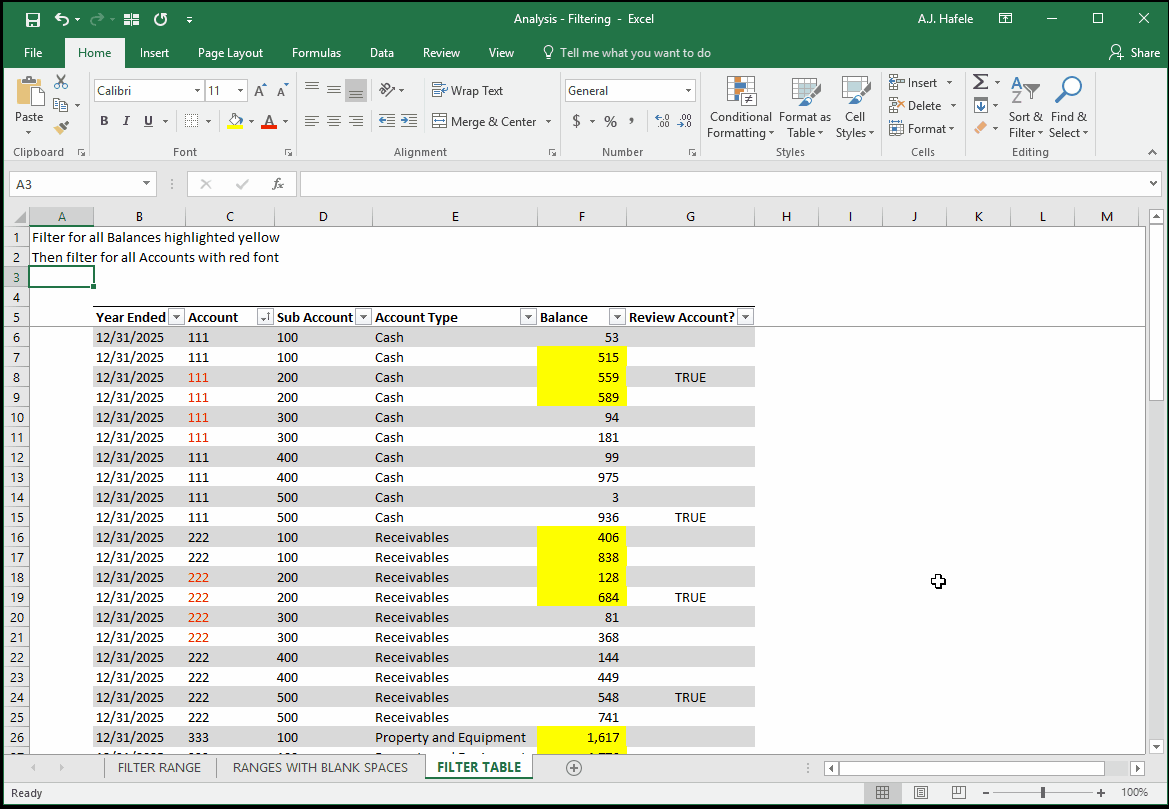
Note that you can also filter by (text or cell) color, as illustrated here:
Filtering by color can come in handy when you are investigating strange items and need to view only that colored data
An even better alternative when dealing with review items, however, is to avoid highlights and simply create a Review field (which is actually what we have done in column G in the above example)
Advanced Filtering
Advanced filtering is another tool that allows you to filter data
Rather than using the filter buttons, you define your filter criteria in a range of cells
Advanced filtering also allows you to copy/paste the filtered results elsewhere in your file
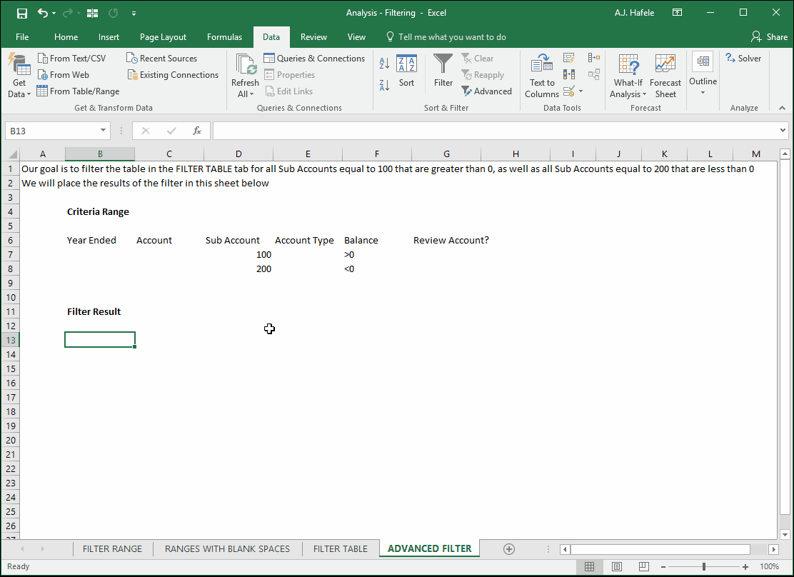
In the examples below, our ultimate goal is to filter for 2 sets of data:
All Sub Accounts equal to 100 whose balances are positive, as well as
All Sub Accounts equal to 200 whose balances are negative
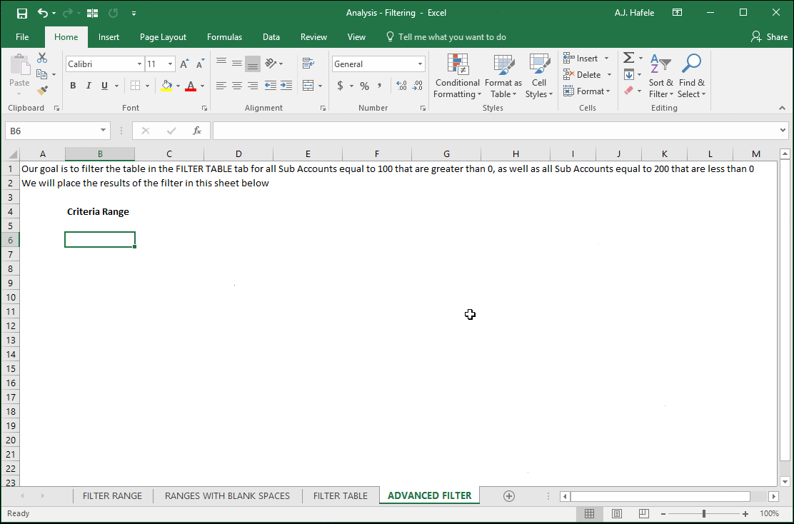
In the first illustration below, we will create our criteria range (in a separate worksheet) by copying and pasting the headers from our table (that we want to filter):
How should we interpret this criteria range?
The first row is the row containing all header names. You will define the criteria directly below the corresponding header names
All items in the same row represent combined requirements (i.e. Sub Account is 100 and the Balance is > 0)
Note that blank values mean that the field can be anything (e.g. since C7 and C8 in the ADVANCED FILTER tab are blank, it does not matter what the Account number is)
Each row represents alternative criteria (i.e. we want to filter for any data which meets the criteria in either row 7 or row 8)
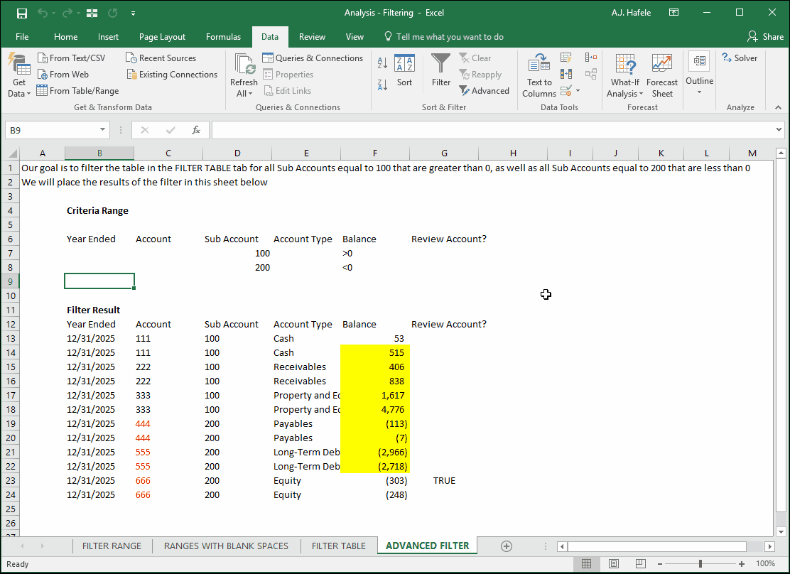
Now, let's apply an advanced filter using the newly-created Criteria Range, and copy the filter results into the ADVANCED FILTER sheet:
A quick word of caution: make sure your Criteria Range does not include a blank row of data (e.g. row 9 in the above example), or else your filter will not work properly (you will end up not filtering anything)
Remember, you can filter the original table (without copying/pasting to another location) by selecting the action "Filter the list, in-place)
Note that when performing an advanced filter, Excel automatically creates two named ranges: "Criteria" and "Extract", as shown here:
These ranges are probably not going to be very useful for you in the future
Last, notice that the Advanced filter menu has a check-box at the very bottom called "Unique records only"
Check this box in the event that you want to purge exact duplicates contained in the table you are filtering (we do not have duplicates in our examples)
By "exact", we mean that every data point in the row is duplicated in another row