If you do not use Excel 2013 or higher (for Windows), you cannot leverage the attached file to follow along, unfortunately (but you can still read through this in preparation for a future Excel upgrade!)
However, this lecture is in-scope for testing, so please read through the material even if you cannot practice
Overview
Starting with Excel 2013, Microsoft has added some useful database-related functionalities to Excel. In particular, you can now create relationships between tables within Excel
What are relationships? In short, they are linkages between tables. Relationships are conceptually similar to VLOOKUP (this will become more clear in the below illustrations)
In this lecture, we will demonstrate how to create a relationship between two tables, as well as how to leverage this relationship to create a multi-table PivotTable
Buttons
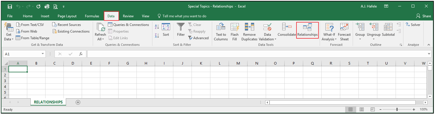
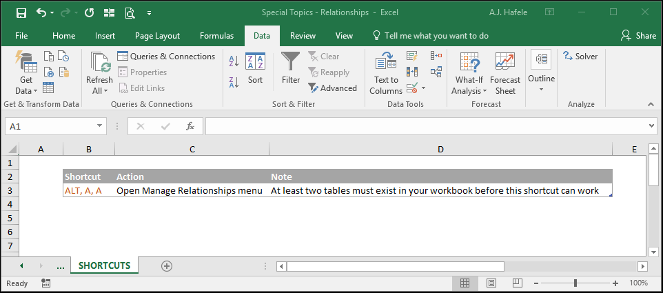
The Relationships button can be found in the Data Tools group of the Data tab:
Example
In the below illustrations, we will be working with two tables:
The _transaction table lists transactions from an accounting system (date, account and amounts are included)
The _accounts table is a list of all accounts in existence, and their corresponding name
Here are the two tables we will be working with:
Our simple goal is to summarize the transactions by Account Name (not account number) in a PivotTable
Summarize Using VLOOKUP
Perhaps the most common way to do this would be to use VLOOKUP and then Pivot the _transaction table, as shown here:
Summarize With Relationships
Perhaps, however, you did not want to use VLOOKUP for some reason
For example, maybe you do not want the VLOOKUP formula to blow up in the future (a legitimate and realistic concern)
As an alternative, you can first create a relationship between the _transaction and _accounts tables, and then you can create a PivotTable with both tables included
In this way, you avoid using any formulas at all
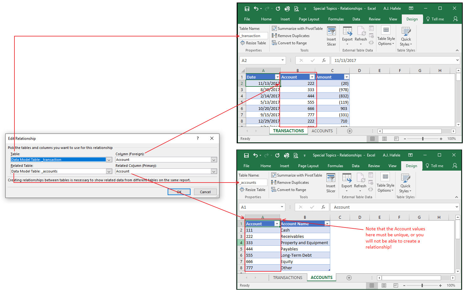
Observe as we first create the relationship between the two tables:
Here is a visualization of the relationship we created:
It is critical to have the proper relationships set up in the Edit Relationships menu, so let's review why we set it up this way:
The Related Table (bottom left) is always your mapping table, which is the table of unique values
The Related Column (bottom right) is the field in your mapping table that you want to associate with a Foreign Column in your Table
The Table (top left) is the table that has at least one field in common with the Related Table
The Foreign Column (top right) is the field that has the same data that is contained in the Related Column
Now, let's create a special PivotTable which includes both tables:
Remember that you must click "Use this workbook's Data Model" when creating your PivotTable (as shown above) for this to work
This produces the same result as in the VLOOKUP example, but with no formulas!
Obviously, the downside is that this method requires a bit more setup versus just using VLOOKUP
Deleting Relationships
To delete a relationship, simply do the following:
As the warning message above indicates, deleting relationships can mess up any structure (such as a PivotTable) that depended on that relationship, so be careful!
Note that you can also modify existing relationships from that menu