By default, a cell (e.g. A1) is named after the cross section of its column letter (e.g. A) and its row number (e.g. 1)
The topmost and leftmost cell in every worksheet is A1
The cell directly below A1 is A2
The cell directly to the right of A1 is B1
The cell one row below and one column to the right of A1 is B2
As you know by now, formulas can be created to reference other cells, such as =A1
More precisely, you can actually use any one of the following formulas and get the same result:
=A1 (this is a relative cell reference)
=$A1 (this is a mixed cell reference)
=A$1 (this is also a mixed cell reference)
=$A$1 (this is an absolute cell reference)
But why are there dollar signs, and what is the meaning of the placement of the dollar signs?
We will answer that question in the discussion below
As you will see, these differences become clear when copying and pasting formulas to different cells
Relative Cell References (=A1)
Using relative cell references is the most flexible way to reference cells, in the sense that both the rows and columns will adjust when the formula is copied and pasted elsewhere
No dollar signs are present in relative cell references (e.g. =A1)
Relative cell references are also the default way of referencing cells
For example, if you select a cell with your mouse or ARROW keys when creating a formula (e.g. selecting cell A1 when creating the =A1+5 formula), relative cell references will appear upon selecting the cell
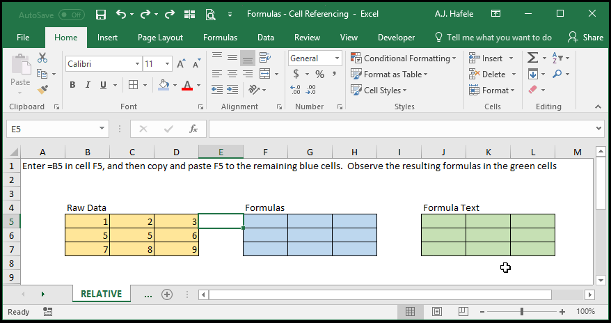
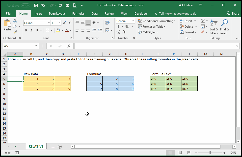
Observe what happens when a formula with a relative cell reference is copied and pasted to multiple rows and columns:
Notice that:
When cell F5 is copied and pasted one row down and one column to the right, to G6, the formula =B5 also adjusted one row down and one column to the right (=C6)!
Also, when we typed =B5 into cell F5, we hit CTRL+ENTER so that we stayed on cell F5, so you can observe the contents in the formula bar (we do this throughout the lecture)
What happens if we were to cut and paste cell B5? Observe the following illustration:
Notice that the output of cell F5 did not change, and the formula in cell F5 (per the corresponding green cell) changed from =B5 to =A5
When cells are cut and pasted, formulas referencing those cells will dynamically change, without regard to the cell referencing type used
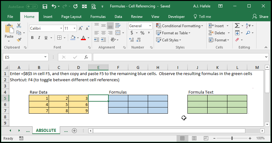
Absolute Cell References (=$A$1)
An absolute cell reference is one that will always refer to the same cell no matter where the formula is copied and pasted
If we need a formula to constantly reference a specific cell no matter where the formula is copied and pasted, we need to "freeze" the reference to both the row and the column
To "freeze" the row and column in a formula, put a dollar sign before both the column reference and the row reference (e.g. =$A$1)
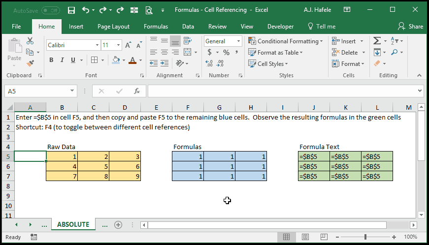
Observe the following illustration, in which an absolute reference (always referencing cell B5) is used:
Notice that:
After we selected B5, we pressed the F4 key one time to change the formula to =$B$5
Pressing F4 multiple times while in Enter Mode or Edit Mode will actually toggle between the four types of cell references, in the following order:
Start with: =B5
Press once (1st time): =$B$5
Press again (2nd time): =B$5
Press again (3rd time): =$B5
Press again (4th time): =B5
Etc.
We use this shortcut in the remaining illustrations (though we may press it more than once, depending on the reference type!)
No matter where we copy and paste cell F5, the resulting formula will be =$B$5
What happens if we were to cut and paste cell B5? Observe the following illustration:
Notice that the output in the blue cells (i.e. 1) did not change, as the absolute references (as shown in the green cells) changed from =$B$5 to =$A$5
Again when cells are cut and pasted, formulas referencing those cells will dynamically change, without regard to the cell referencing type used
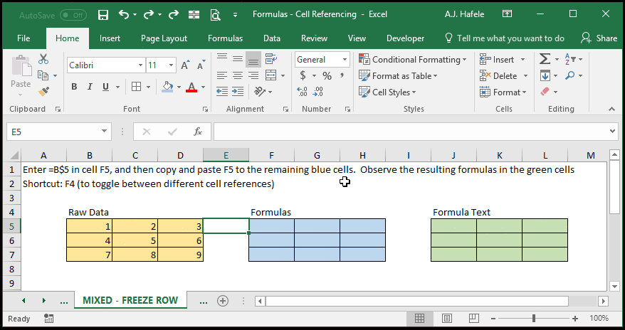
Mixed Cell References - Frozen Row (=A$1)
A mixed cell reference:
Is a hybrid between a relative and absolute cell reference
Always has a single dollar sign in the cell reference
Is written such that the dollar sign is placed either before the column letter only, or before the row number only
If we need a formula to constantly reference a specific row no matter where the formula is copied and pasted, we need to "freeze" the reference to the row
To "freeze" only a row in a formula, simply put a dollar sign before the row number (e.g. =A$1)
Observe the following illustration, in which a mixed reference (always referencing row 5) is used:
Notice that:
After we selected B5, we pressed the F4 key two times to change the formula to =B$5
The rows were frozen, so row 5 was always referenced
The columns were not frozen, so only 1, 2, or 3 (in row 5) was referenced in each column
Though not shown, cutting and pasting a yellow cell would work in the same manner as shown above. That is, the formulas in the blue cells will adjust to reference the new location of the yellow cells, regardless of the cell reference type used
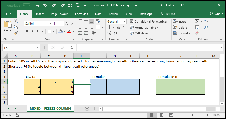
Mixed Cell References - Frozen Column (=$A1)
If we need a formula to always reference a specific column no matter where the formula is copied and pasted, we need to "freeze" the referenced column
To "freeze" only a column in a formula, simply put a dollar sign before the column letter (e.g. =$A1)
Observe the following illustration, in which a mixed reference (always referencing column B) is used:
Notice that:
After we selected B5, we pressed the F4 key three times to change the formula to =$B5
The columns were frozen, so column B was always referenced
The rows were not frozen, so only 1, 4, or 7 (in column B) was referenced in each row
Though not shown, cutting and pasting a yellow cell would work in the same manner as shown above. That is, the formulas in the blue cells will adjust to reference the new location of the yellow cells, regardless of the cell reference type used
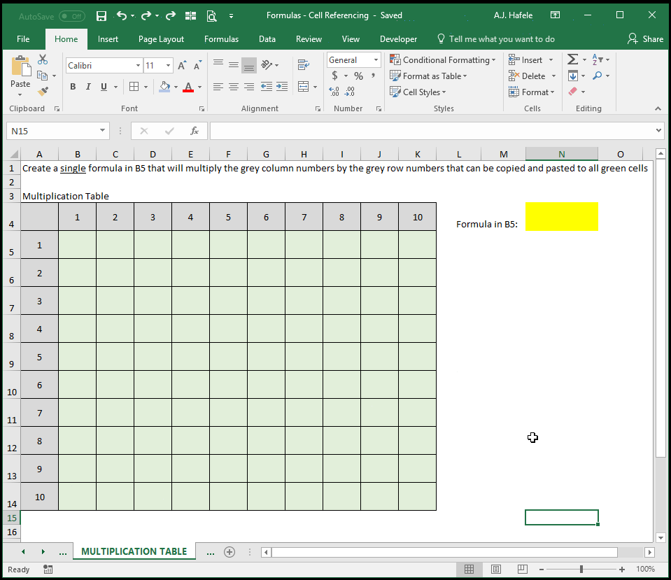
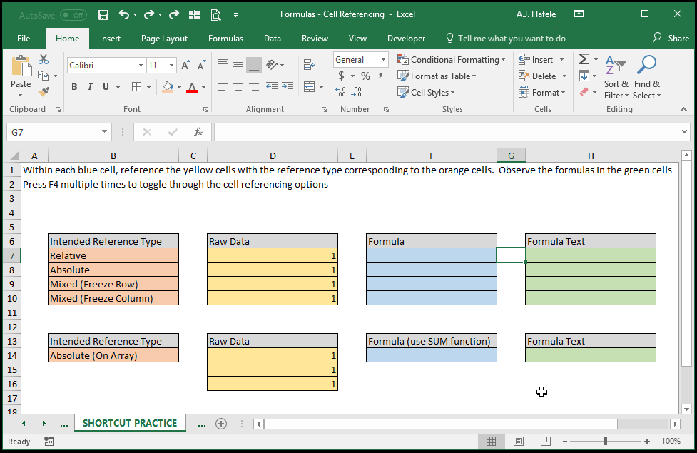
More Practice
The following illustrates how to use the two types of mixed references to quickly create a multiplication table
Notice that:
The first number in the multiplication calculation always references row 4, so we freeze that row (e.g. B$4 in =B$4*$A5)
The second number in the multiplication calculation always references column A, so we freeze that column (e.g. $A5 in =B$4*$A5)
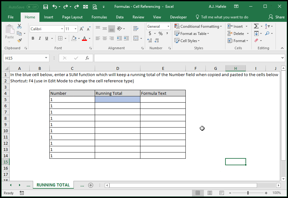
The next example illustrates how to use both absolute and relative cell references in a single array (or range) of cells with the SUM function:
Notice that:
We were able to use an absolute cell reference for the first part of the range (e.g. =SUM($C$5:C5), and a relative cell reference for the second part of the range (e.g. =SUM($C$5:C5)
In order to change the first C5 to an absolute cell reference, we had to select just that part of the range with the cursor
When copied and pasted down, cell C5 is always referenced as the first (or starting) cell in the range, since it has an absolute reference
Likewise, each cell in column C in each row in is referenced as the last (or ending) cell in the range, since it has a relative cell reference
We could have also used the mix reference C$5 instead of $C$5 as the first reference in the range, to arrive at the same output
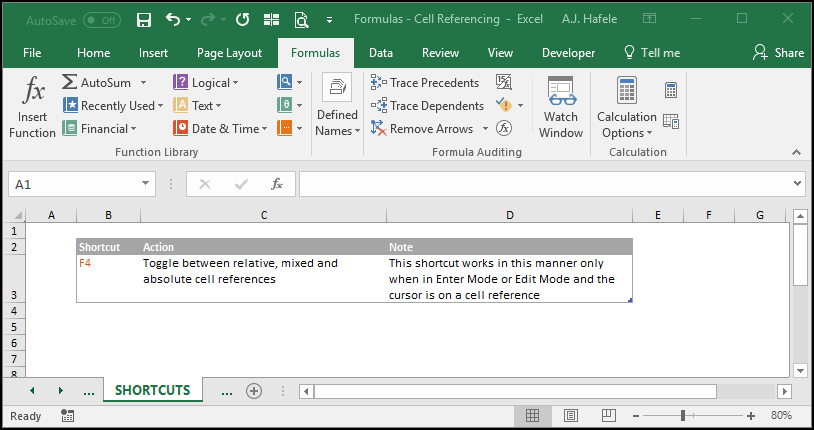
Shortcuts
As you have seen throughout the lecture, the F4 shortcut is a very fast and easy way to toggle through the four types of cell references
When in Edit or Enter mode, simply select the cell reference in question and press F4, as shown here:
Notice that:
When using SUM to add D14:D16, we pressed F4 once, and the entire array switched to absolute cell references!
But remember, if you need to change the reference type on just a part of an array (e.g. cell D14 only, rather than D14:D16), select that part with your cursor and then use F4 (as used to create the running total calculations in the earlier illustration)
Be sure to use F4 often to improve your efficiency
Tips
Get comfortable with all possible ways to reference cells
Make frequent use of relative, absolute, and mixed cell references to enhance the flexibility of your Excel files
Conversely, make it a habit to avoid the use of hard-coded data in formulas