Thus far, we have covered how you can "hard-code" formats (e.g. how to highlight a specific cell yellow)
But what if we need to apply formatting only when cell contents meet certain conditions (e.g. highlight a cell yellow if the value is greater than 100)?
The answer: use conditional formatting!
Conditional formatting is a feature that automatically formats cells whose contents meet certain user-defined conditions (hence the name!)
As discussed below, you have the the ability to use either pre-defined or custom conditional formatting rules
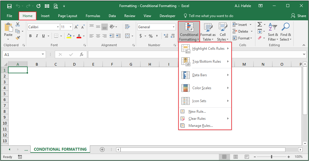
Buttons
The relevant buttons can be found in the Styles group of the Home tab:
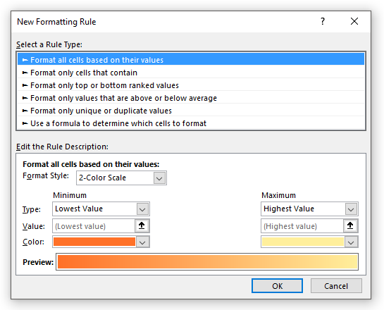
When the New Rule... button (above) is selected, the New Formatting Rule menu appears:
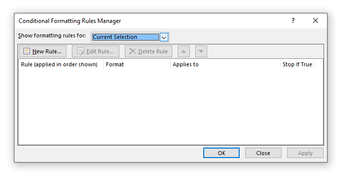
When the Manage Rules... button (in the first screenshot above) is selected, the Conditional Formatting Rules Manager menu appears:
We will show you how to use these buttons and menus in the below discussion
Highlight Cell Rules
Let's jump right in to the various conditional formatting options available via the Ribbon
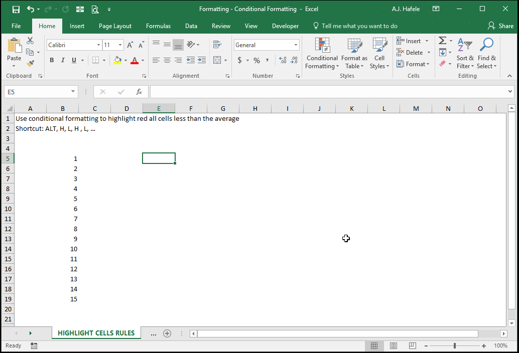
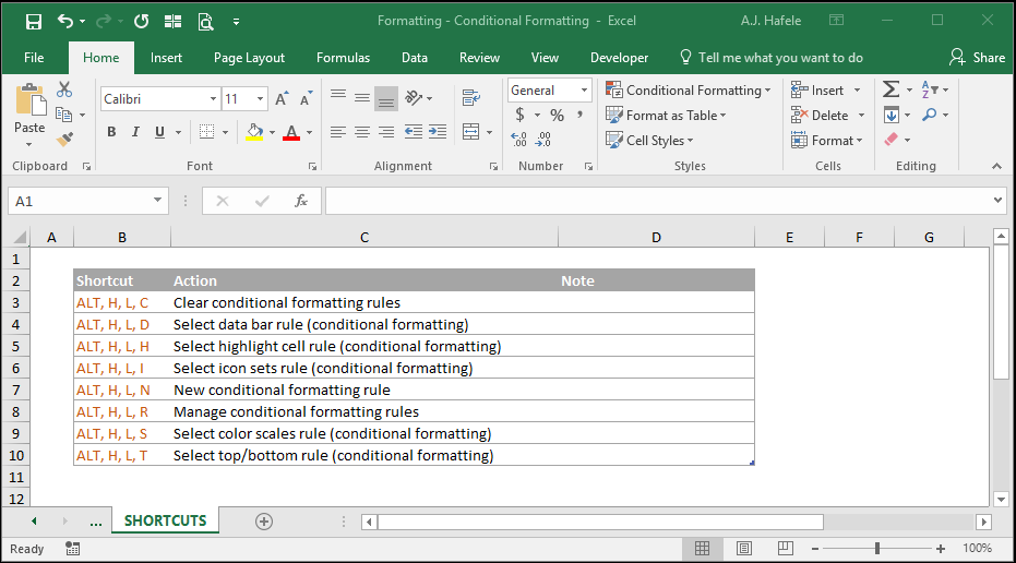
The following illustrates how to highlight (red) values less than the average of the set (using the AVERAGE function) via the Highlight Cells Rules sub-menu (ALT, H, L, H):
Notice that, upon changing the value in B19 from 15 to -10, the red highlights automatically change to capture the applicable cells
This simple example shows you the power of conditional formatting - the formatting is applied in a dynamic fashion, changing as underlying data are changed
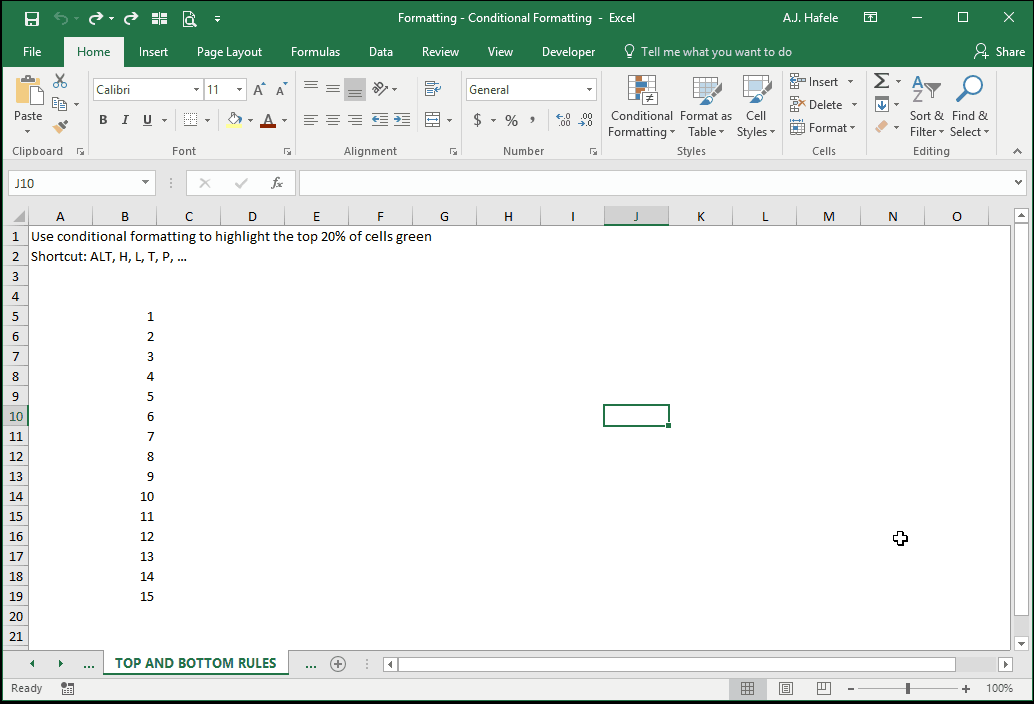
Top/Bottom Rules
The following illustrates how to highlight green the top 20% of cells (in terms of value) via the Top/Bottom Rules sub-menu (ALT, H, L, T):
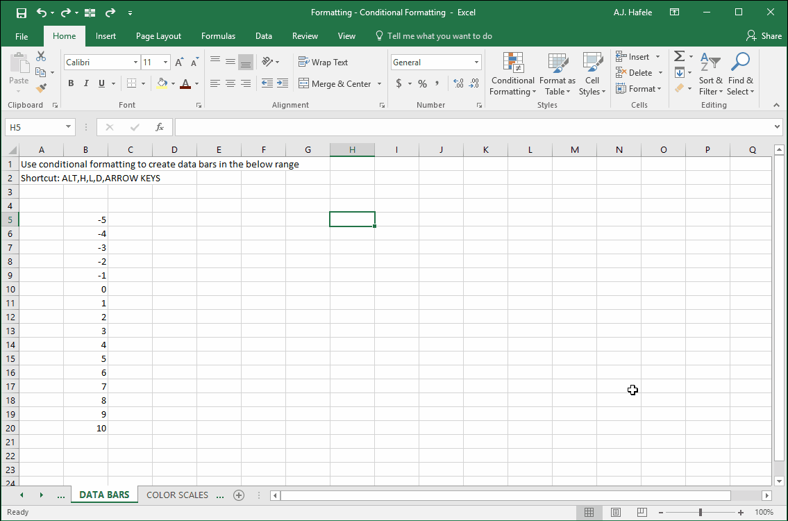
Data Bars
The following illustrates how to add data bars to a range of cells (to better visualize relative values) via the Data Bars sub-menu (ALT, H, L, D):
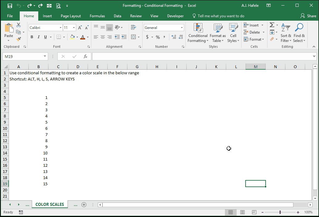
Color Scales
The following illustrates how to add color scales to a range of cells (to better visualize relative values) via the Color Scales sub-menu (ALT, H, L, S):
Although not shown above, the colors will dynamically adjust as the relative values change
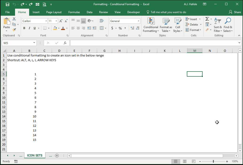
Icon Sets
The following illustrates how to add an icon set to a range of cells (to better visualize relative values) via the Icon Sets sub-menu (ALT, H, L, I):
Although not shown above, the icons will dynamically adjust as the relative values change
(Custom) Formula Rule
If none of the pre-defined conditional formatting rules are adequate, you have a lot of flexibility in creating custom rules
To create a custom rule on a range of cells, you simply write an equation or inequality that, if TRUE, formats your range in any manner you wish
Note that you can use functions when creating your equation or inequality
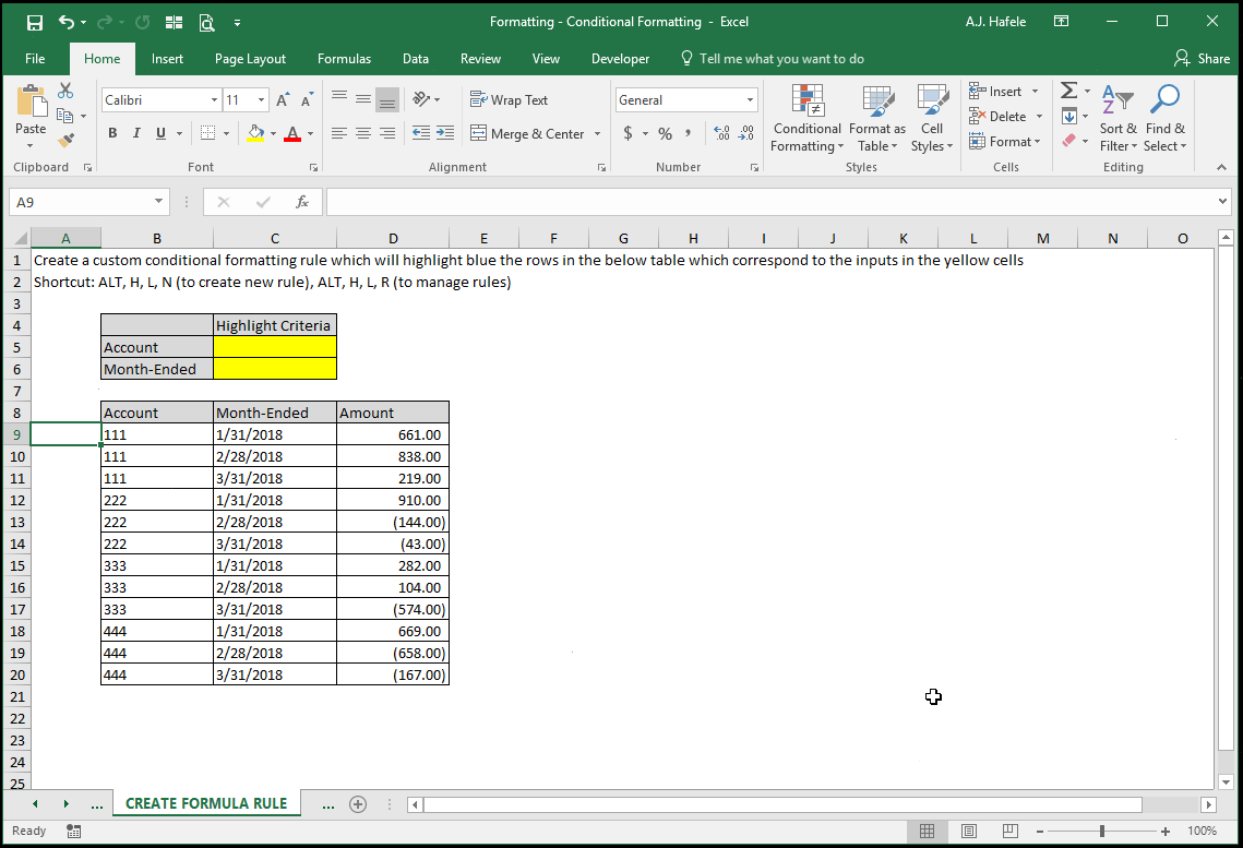
In the next illustration, we create a custom rule that will highlight rows blue if two user-defined inputs (in the yellow cells) are found in any row within the selected range
Importantly, it is crucial to keep in mind that conditional formatting rule formulas should be written from the perspective of the active cell (B9 in this example):
Note that we have not seen the conditional formatting in action yet; we need to first discuss the formula itself
Carefully observe the rule's formula in B9 =AND($B9=$C$5, $C9=$C$6)
Why did we use the AND function?
We used AND because we needed two conditions to both be TRUE:
The value in column B of the data (Account) should match C5 (in yellow)
The value in column C of the data (Month-Ended) should match C6 (in yellow)
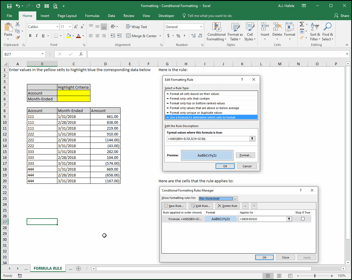
Why did we use absolute and mixed cell references in the formula?
First, you must imagine that you were writing this formula where the active cell is (cell B9 in this instance), directly into the cell
Next, imagine that you copy and paste this formula to all cells in the range of data (containing the account numbers, dates and amounts)
C5 and C6 are absolute references because they will need to be referenced in each cell upon copying and pasting
Columns B and C need to be referenced each time upon copying and pasting, as those columns contain the values corresponding to the yellow inputs (Account and Month-Ended)
After the (imaginary) copy and paste, each cell will either say "TRUE" or "FALSE"
In this hypothetical situation, conditional formatting will only apply to the cells that have a value of "TRUE"
If you do not yet understand, no worries - we will illustrate below
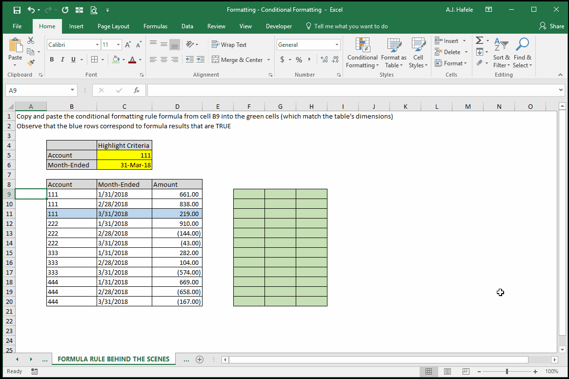
But first, observe the actual results of the rule, as we add values to the yellow cells:
Wait - how is this working, again? As discussed above, conditional formatting is applied only to those cells whose conditional formatting formula values (that were hypothetically copied and pasted) are TRUE:
In the above example, we copied and pasted B9's rule to the right of the table (rather than directly over it) to illustrate the parity between the blue highlight and the TRUE values in the copied/pasted formulas
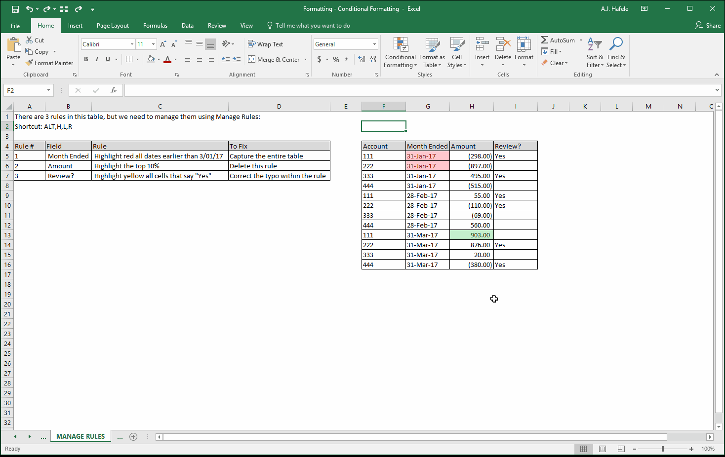
Manage Rules
Existing conditional formatting rules can be managed in the Conditional Formatting Rules Manager menu, which allows you to modify rules, delete rules, and/or change the cells subject to those rules, as shown here (ALT, H, L, R):
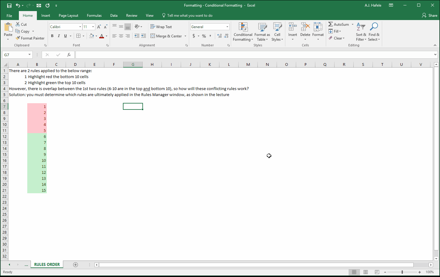
Rules Order
What happens if two or more different rules apply to the same cell? What will the format be? Excel lets you choose!
The Conditional Formatting Rules Manager window allows you to specify the order in which the rules apply
As shown in the next example, the top 10 of 15 cells are highlighted green, and the bottom 10 of 15 cells are highlighted red, so 6-10 are subject to both rules
In Conditional Formatting Rules Manager menu, you can specify the order in which the rules apply, with the topmost rules being applied first, and the bottom rule being applied last:
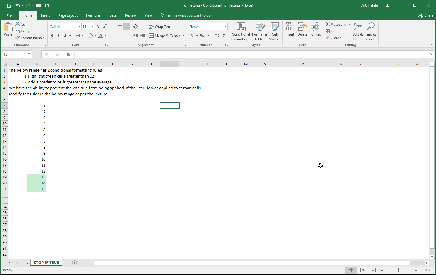
Additionally, you can stop all future conditional formatting rules from being applied, once a rule is initially applied to a cell, by checking "Stop if True" next to the applicable rule, as shown here:
Notice in the above example, if we check the "Stop if True" box on the topmost rule, the rule below it is no longer applied (where both rules would have applied to a given cell)
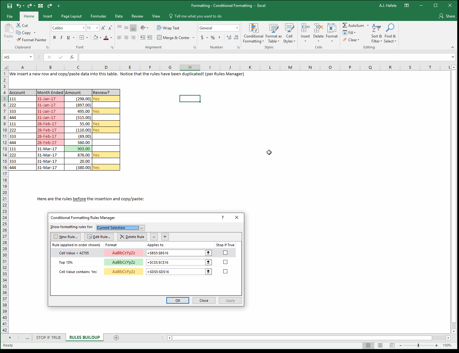
Rules Buildup
There is one major problem to be aware of when using conditional formatting rules - copying/pasting and inserting/deleting data where conditional formatting rules are applied can create duplicates of the same rules (which we refer to as "rules buildup")
The following example illustrates the duplication of conditional formatting rules when a new row is inserted and data are copied/pasted into that row:
Over time, these duplicate rules can build up and make conditional formatting more difficult to manage
Rules buildup can also make your file slower
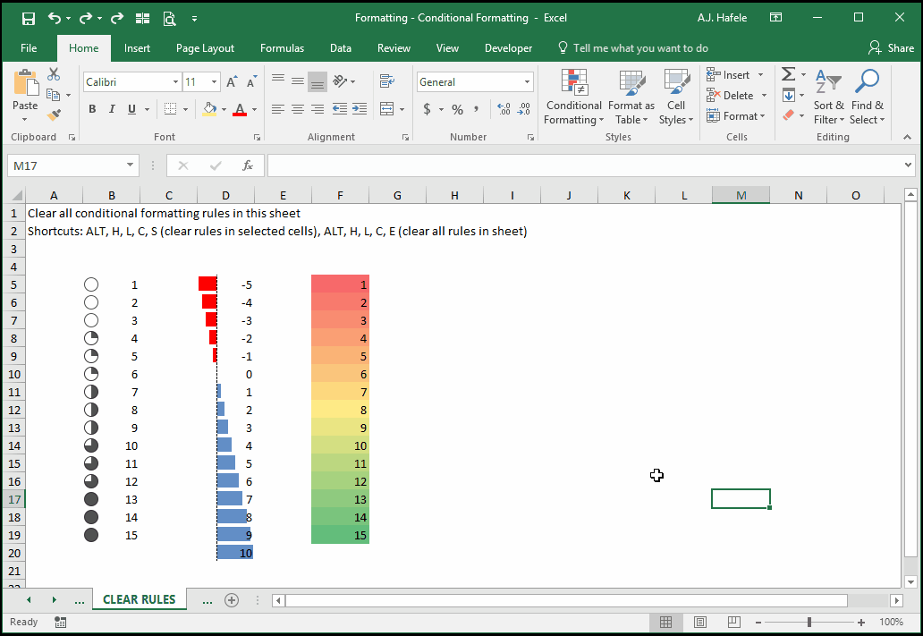
Clear Rules
The following demonstrates how to clear (i.e. remove) conditional formatting rules from a worksheet (ALT, H, L, C):
Tips
Use conditional formatting rules with only where necessary
Avoid using conditional formatting rules in tables in which copying/pasting and insertions/deletions are common, to avoid rules buildup
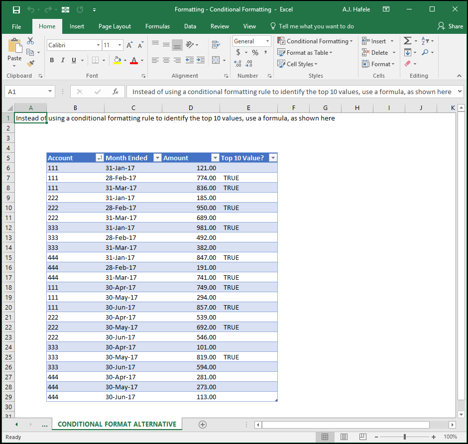
If you are using conditional formatting to flag certain data in a table, consider instead adding a field that flags items, as shown here:
This might not look as cool, but utilizing a separate field is typically easier to manage (and you do not have to worry about rules buildup)