This lecture is very important, so read carefully and you will take away a lot of useful info!
This is one of the most important lectures in the entire course
If you are not using tables, you might not be doing your work as efficiently as you could
Overview
This lecture covers tables (or "Excel tables"), which are used to manage tabular sets of data
Importantly, tables are not simply ranges of data contained in your worksheets
Rather, tables are unique objects used to store data and make calculations, but they also come with many useful features that are not available in normal ranges of data
As such, the topic of tables spans beyond formatting alone (we could have placed this lecture in the Editing or Analysis course sections)
As a brief side note, be aware of terminology nuances: there is a difference between tables (discussed in this lecture) and data tables (discussed later)
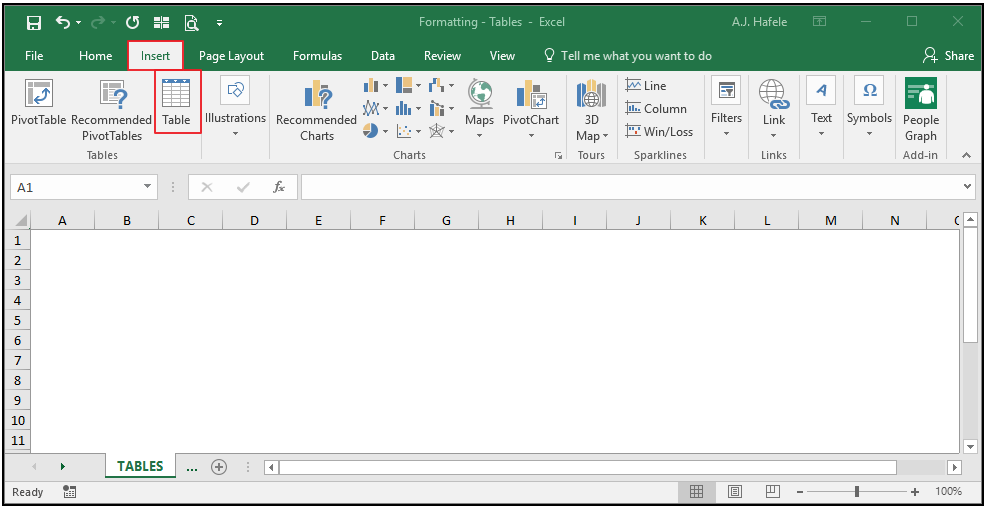
Buttons
The relevant button can be found in the Tables group of the Insert tab:
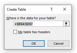
When that button is pressed, the Create Table menu appears:
As you can see, the only inputs in this menu are 1) the range of cells to be converted into a table, and 2) whether or not that range has headers (or column names) already
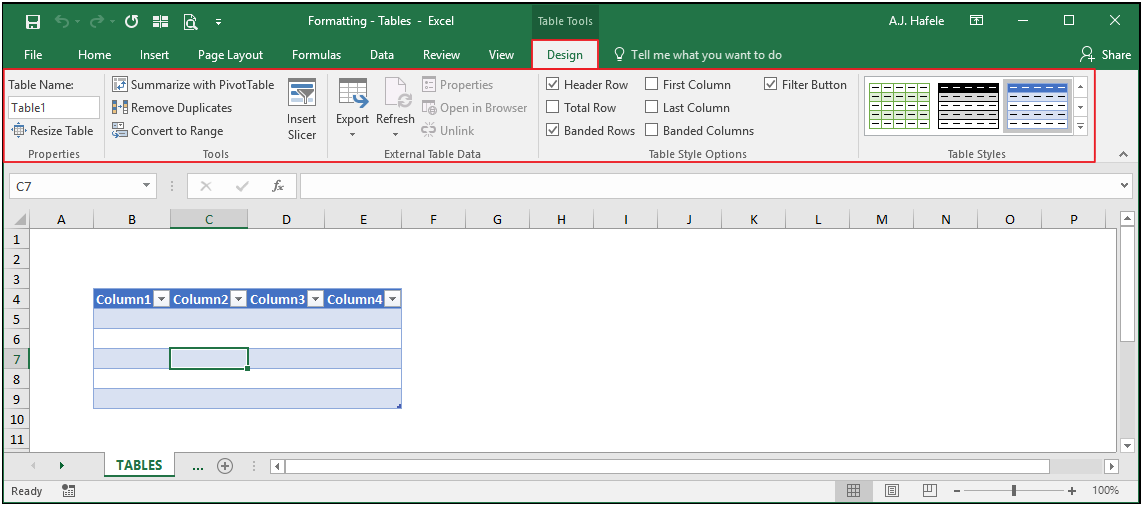
Moreover, after a table is created and the active cell is anywhere in the table, an entirely new tab in the Ribbon - Design - is available, with a multitude of options:
We will explore these menu options in more detail below
Create Table
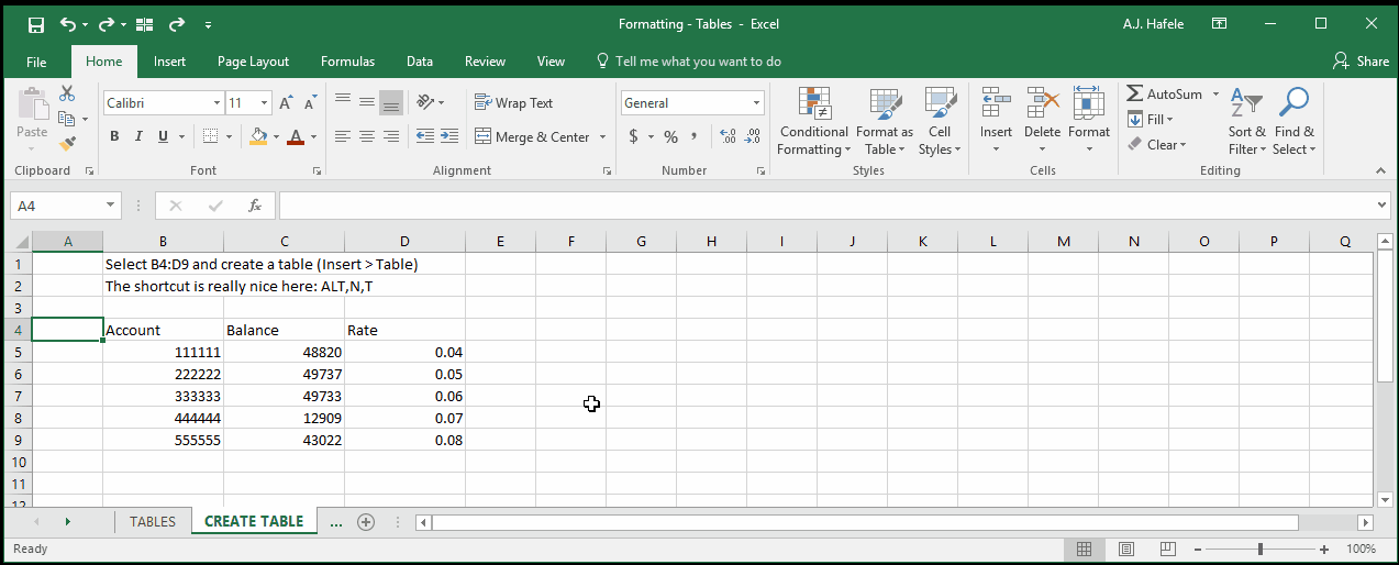
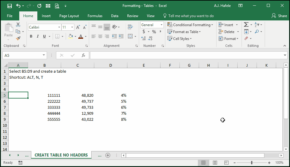
Let's begin by showing you how to create a table - it's easy!
Observe as we convert a normal range of data to an Excel table (ALT, N, T or CTRL+T):
Notice that:
Since the range we selected already included headers (Account, Balance, and Rate), we need to ensure the "My table has headers" option is checked within the Create Table menu
Excel automatically detected that we had headers and checked the box for us, but that may not always be the case
Immediately after creating the table, the Design tab became available in the Ribbon
A table name is automatically generated (Table17, as per the left end of the Design tab)
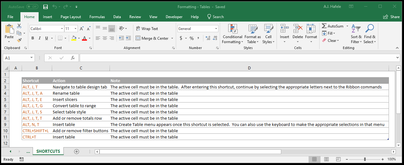
You can change the table name within the Design tab if desired (ALT, J, T, A)
If our range did not have headers, Excel would create generic headers for us, as shown here:
Notice that:
Generic field headers were created after inserting the table
Each field name is unique; you can never have two field headers that are exactly the same
Excel prevents duplicate fields names by appending numbers to field names
We will discuss why this is necessary in the section on structured referencing below
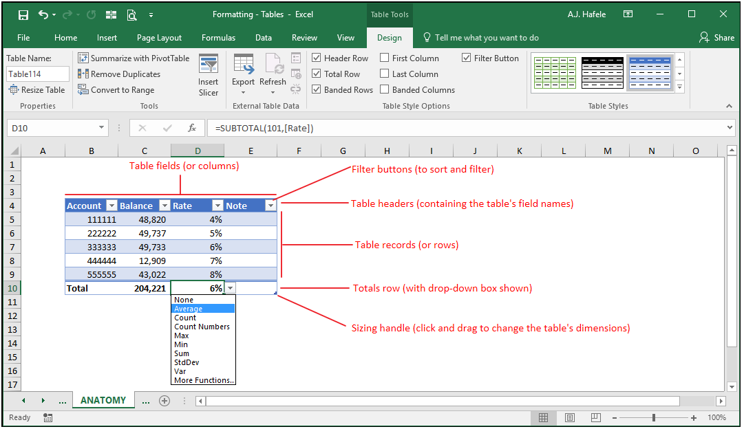
Anatomy of a Table
Now that you know how to create tables, let's review their components:
Table fields (or columns):
These are the vertical columns of similar data which make up your table
Ideally, all information in a given field is formatted exactly the same (e.g. all rows in the Rate field are percentages)
Ideally, if a formula is used in a field, a single formula should be used for each record in that field
However, this is not a requirement
Remember that each field name (or header) must be unique!
Filter buttons:
These buttons, located on each field header, allow you to rearrange and filter data (sorting and filtering are discussed later in the course)
You can remove these buttons via the Design tab, if desired (CTRL+SHIFT+L when active cell is in the table)
Table headers:
This is always the topmost row in your table, which is intended to hold field names, which describe the data contained in their columns
Again, you can never have duplicate headers (having duplicate headers would be equivalent to having two column A's)
Moreover, you cannot use formulas in headers
Table records (or rows):
This is where your data are stored
All data on any given record should correspond to one another (e.g. Account 222222's balance is 49,737, and its rate is 5%)
Totals row (or "total row"):
This is an optional row at the very bottom of your table which provides summary information on your table
You can add or remove a totals row in the Design tab (ALT, J, T, T)
A drop-down box is available which lets you choose what calculation to make (the SUBTOTAL function is used)
SUBTOTAL is used because (as discussed later) it will calculate subtotals only on filtered data
Note, however, that you can actually enter custom text or formulas in this row, if necessary
Sizing handle:
This handle allows you to increase (or decrease) the dimensions of your table
Clicking and dragging it right (left) will add (delete) fields
Clicking and dragging it down (up) will add (delete) records
Importantly, when fields or records are deleted, the data are not deleted, but they are no longer in the table
We will demonstrate how these components work in more detail below
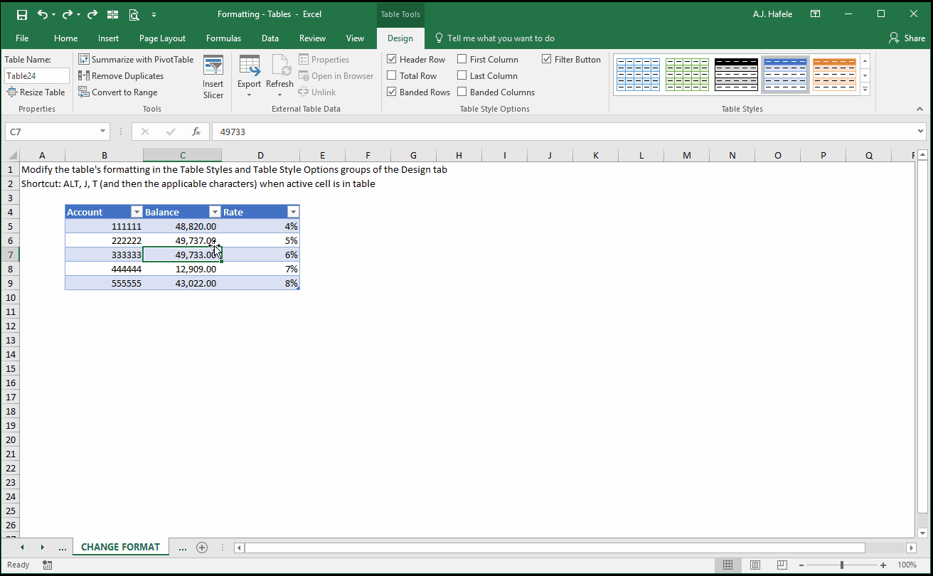
Change Table Format (Style Options)
What if we want to change how our table looks, in terms of colors, borders, shading, etc.?
Easy! The Design tab has plenty of styling options to choose from
Observe as we modify the style of our table:
Be sure to use these options to enhance the clarity and organization of your data
Stop and think about one simple - yet major - advantage here: by creating a table and using built-in style options, you don't have to worry so much about creating and managing your own borders, colors, etc. This can save valuable time and effort!
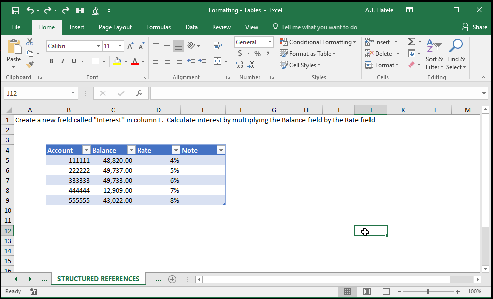
Table Formulas and Structured References
Let's move on to another important aspect of Excel tables - structured references
"Structured referencing" is the term used to describe how cells (and ranges of cells) are referenced within tables
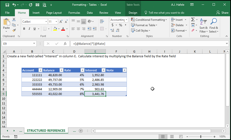
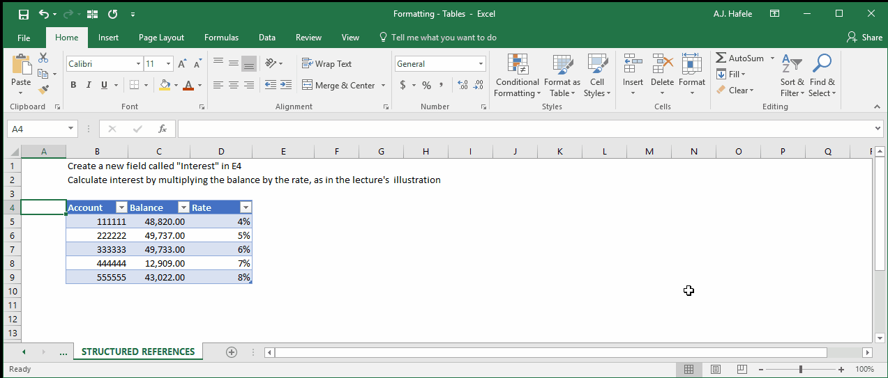
To make this easy to understand, let's jump into a demonstration by adding a new field - Interest - in our table from previous illustrations
Interest is calculated with a simple formula (=Balance * Rate), as shown here:
Notice that:
The resulting formula in cell E5 was not =C5*D5
Rather, formula was =[@Balance]*[@Rate], which is actually more intuitive, since you can tell what information is being multiplied together
The exact same formula was automatically applied to every record in the Interest field after we hit ENTER in cell E5
Why does this formula work, even though we do not reference cells by their rows and columns?
As you might have guessed, Excel knows that each row in the table (e.g. row 5) contains data points of some similar thing (e.g. row 5 contains all data for Account 111111, including the account number itself)
Given this fact, all you need to do is specify the field names in your formulas (e.g. Balance and Rate), and Excel knows which cells need to be referenced in your formula (e.g. the intersection of row 5 and the Balance and Rate fields)
The point above explains why you can never have duplicate field names. If you had two "Account" fields within a single table, for example, Excel would not know which of the two to reference!
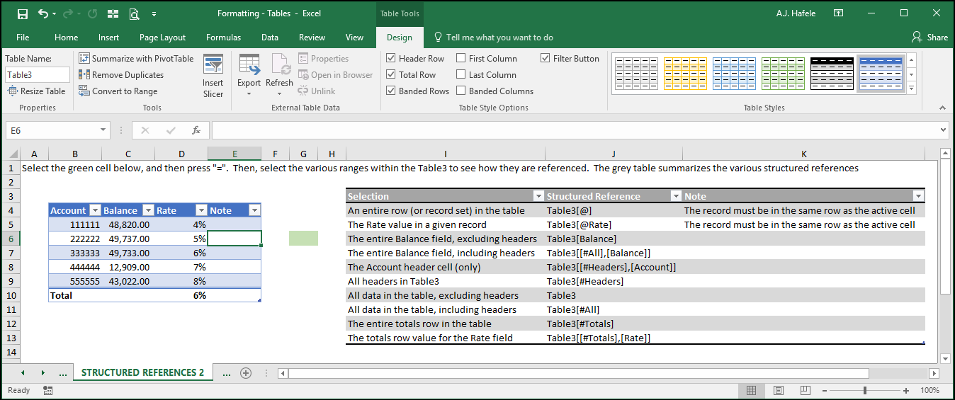
The below screenshot includes a table which presents examples of the different structured referencing conventions available (column J):
Keep in mind that memorizing this syntax is not necessary!
If you ever need to reference certain parts of a table, simply select that part with your mouse or keyboard, and the proper references will be generated automatically
Importantly, you can indeed use structured references outside of tables (in normal ranges) to reference data contained within tables
Note, however, that you can still use standard cell references (e.g. =C5*D5), as shown in the following example:
As shown above:
You must type the cell references rather than select the cells with your keyboard or mouse for this to work
The formula was (again) applied to each row in the Interest field, with references dynamically changing
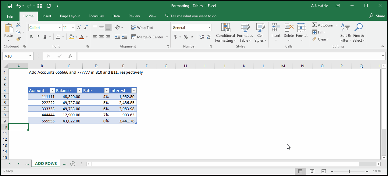
Add New Records
Observe as we add new records by typing directly below the table:
Notice that:
The table automatically detected new record entries and expanded the table downward
The cell formats were copied down to the new records (e.g. the rates stayed in percentage format, the interest figures stayed in the accounting format, etc.)
The Interest formula was copied down automatically when the new records were added
This will not work with idiosyncratic formulas, however
Add New Fields
Observe as we add new fields by typing in a cell directly to the right of the table:
By entering content directly to the right of the table, the table automatically expanded right one column
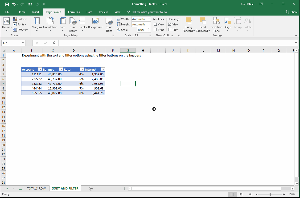
Sort and Filter Within Table
When a table is created, filter buttons are automatically placed on the headers, though they can be removed via the Design tab
Use these buttons to sort and filter your table, as shown here:
We will discuss sorting and filtering in more detail later in the course
Note that you can indeed sort and filter data that are not in a table, but using a table to sort and filter is advantageous, since you will always know exactly what is subject to sorting and filtering (i.e. the data within table itself)
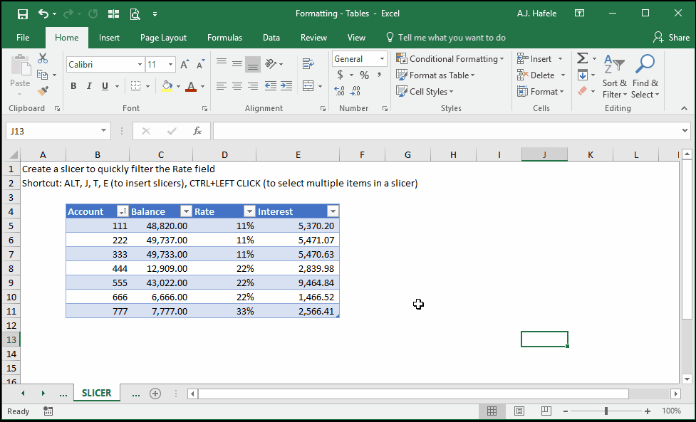
Slicers
Slicers are essentially buttons that allow you to quickly filter fields, as shown here (ALT, J, T, E):
As shown above, there is not much of a difference between using slicers and the filter buttons, except that your filters are more visible
Totals Row
What if you need to summarize your table's data in some way (e.g. sum, average, maximum, minimum, etc. of each field)?
Easy - simply add a totals row to your table, as shown here (ALT, J, T, T):
Look closely at the formula in the totals row above - it is a SUBTOTAL function which calculates totals based on visible cells only
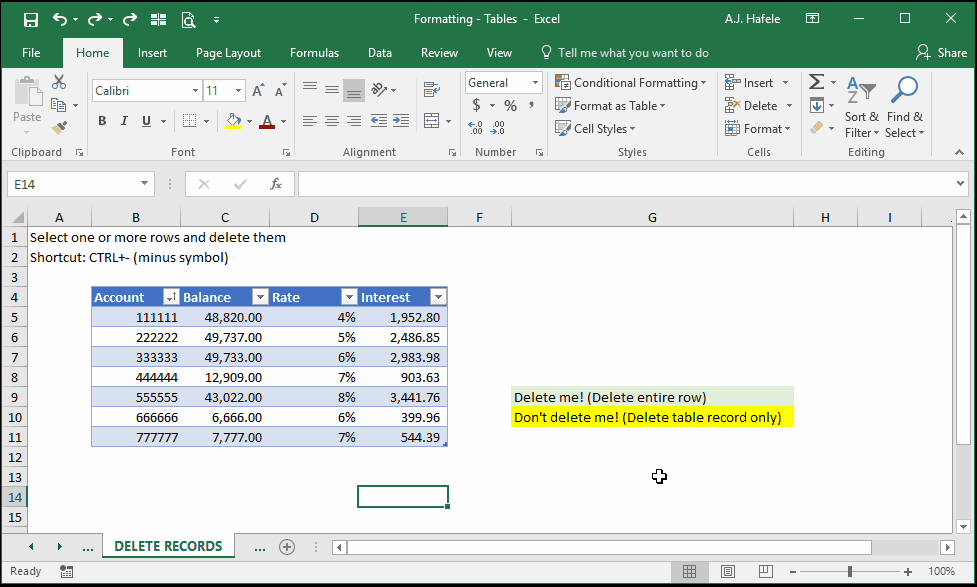
Delete Records
The following illustrates a number of ways to delete records from a table:
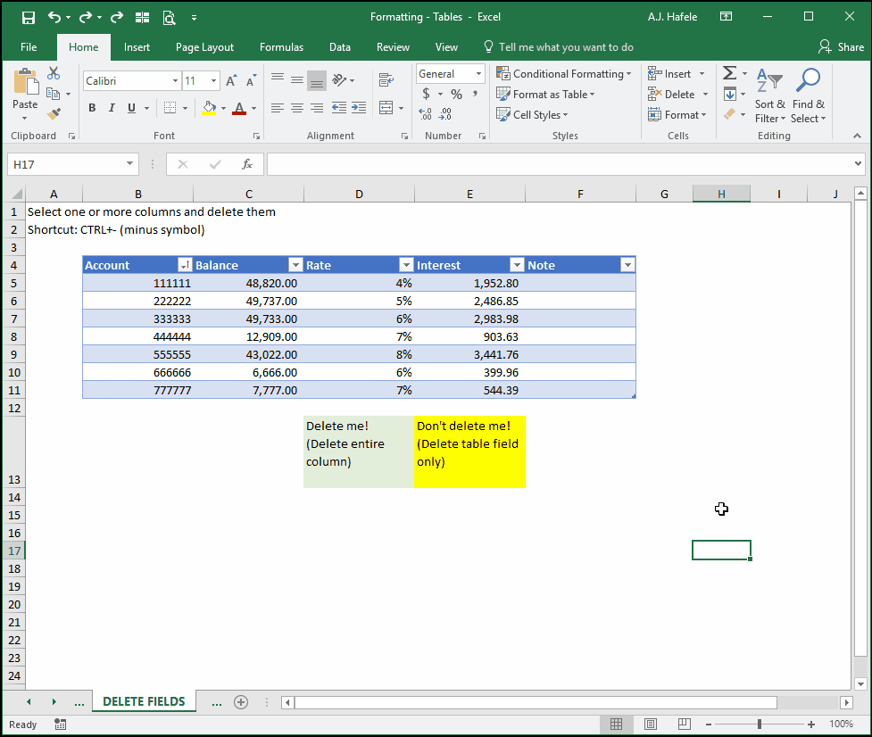
Delete Fields
The following illustrates a number of ways to delete fields from a table:
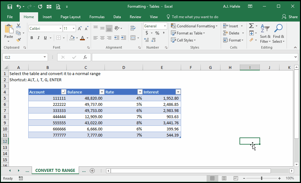
Convert Table to Range
If you decide that you no longer need to use an Excel table, you can convert it back to a normal range of data, as follows (ALT, J, T, G):
Notice that:
The Design tab is no longer available after converting to a range
Immediately after converting to a normal range, the formatting (the borders and colors) did not change
We can modify the formatting of the range, since it is no longer a table
Excel Relationships
Excel 2013 and higher enables us to create relationships between two or more tables
Relationships are essentially connections between separate tables of data
Note that the use of tables is required in order to create relationships in Excel!
Tables With PivotTables
We discuss PivotTables in more detail later, but just know that they are used to analyze/summarize data in a very flexible manner
If you use PivotTables often, always keep your underlying data in a table!
Note that you can create PivotTables on normal, non-table ranges (but we do not recommend doing this!)
By keeping your data in a table, you do not have to continuously (and manually) update your data source (the range of data that you are analyzing)
In other words, if you add new records to your table, all you need to do is refresh your PivotTable to update it
Tips
Tables may be one of the most underused (yet powerful) tools in Excel, from the author's experience
To quickly review, here are some advantages of using Excel tables:
The effort to style your data (and maintain that style) is minimal with Excel's pre-defined table formats
Structured references can make it easier to understand complicated formulas
The totals row eliminates the need to create and maintain your own summary row
You no longer have to worry about dragging down formulas when adding new raw data, assuming consistent formulas are used
You can create relationships between tables, enhancing your analytical capabilities
Tables make using PivotTables much more manageable by no longer requiring you to update the source data range
Think about it - after structuring your table and writing any necessary formulae, all you need to do is simply maintain the raw data, and Excel handles almost everything else!
Make it a habit to use Excel tables when working with tabular data sets and PivotTables