The PivotTable is one of Excel's most powerful tools for analyzing data
PivotTables are very popular because they allow you to slice and dice data very quickly and efficiently
As such, understanding how PivotTables work is vital in making the most of Excel
In this lecture, we will cover a broad range of topics, including (but not limited to) the following:
Organizing source data
Creating and structuring PivotTables
Sorting, filtering, and grouping data
Changing PivotTable styles / layouts
Modifying PivotTable options
Refreshing PivotTables
Using PivotCharts
Though we cannot cover all aspects of PivotTables, we are confident that this lecture will help you grasp the most important concepts
Warning! This is perhaps the longest lecture in the entire course, so take a deep breath, and then proceed!
We highly recommend following along by using the attached Excel file and replicating what we do in each illustration below
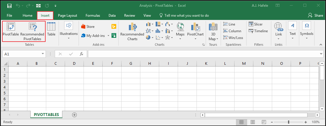
Buttons
The relevant buttons (used to create PivotTables) can be found in the Tables group of the Insert tab:
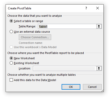
When the PivotTable button is selected, the Create PivotTable menu appears:
This menu allows you to define your source data range, as well as the target location of your PivotTable (among other options)
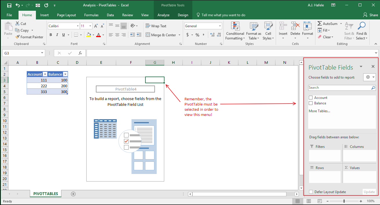
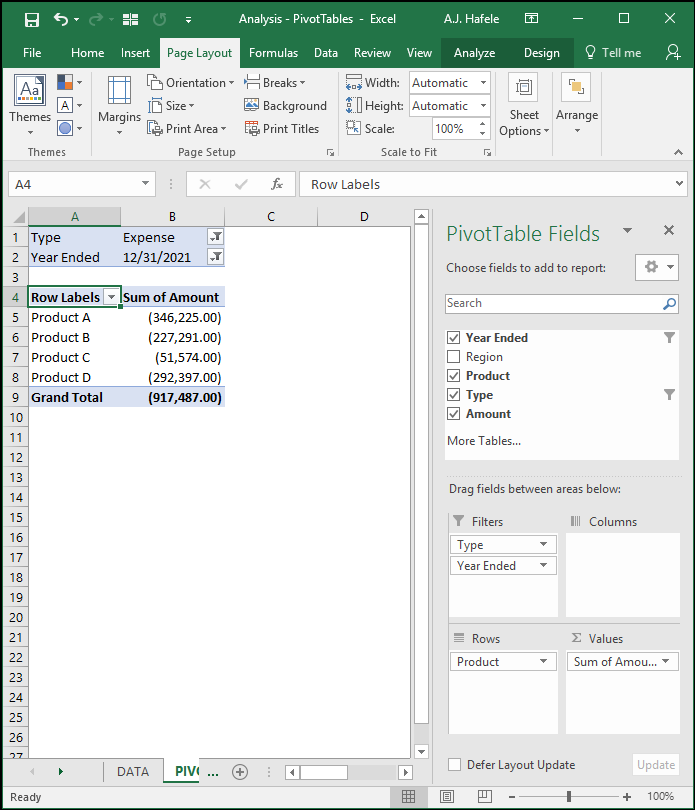
Once a PivotTable is created, the PivotTable Fields menu becomes available once the PivotTable area is selected, as shown in this screenshot:
Below, we will discuss how to create PivotTables, as well as how to utilize the PivotTable Fields menu
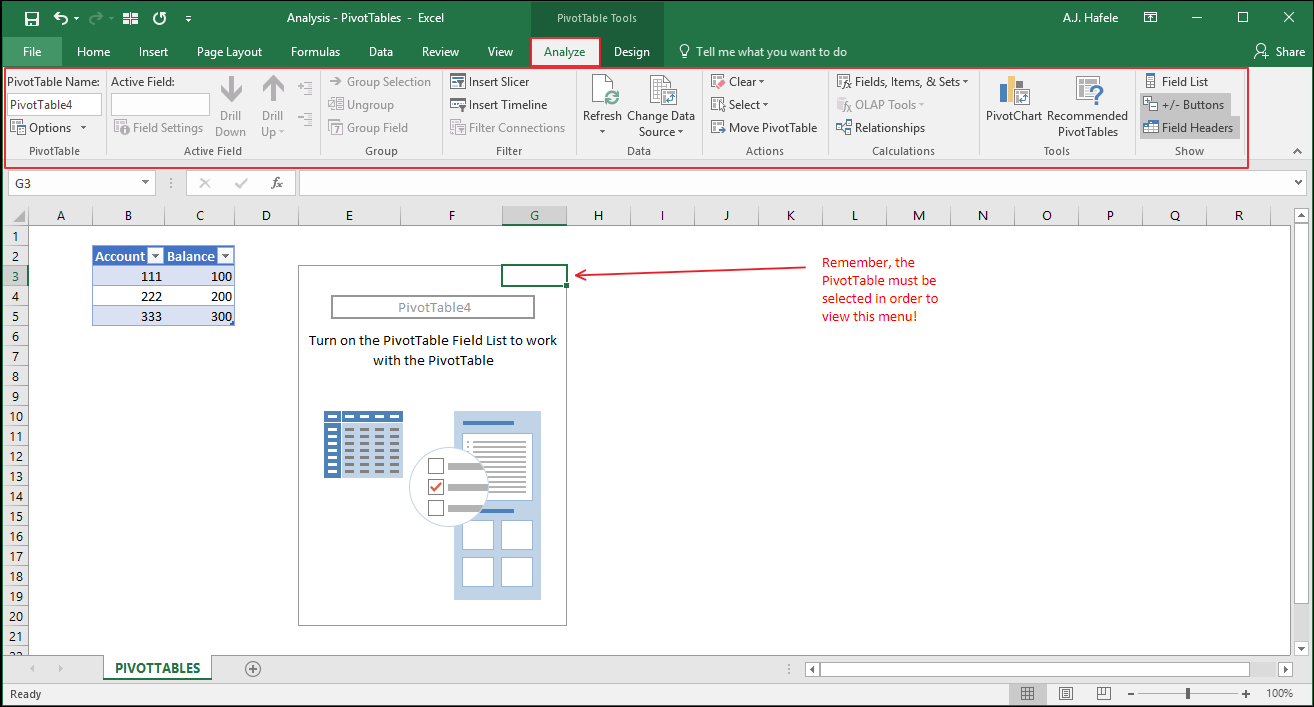
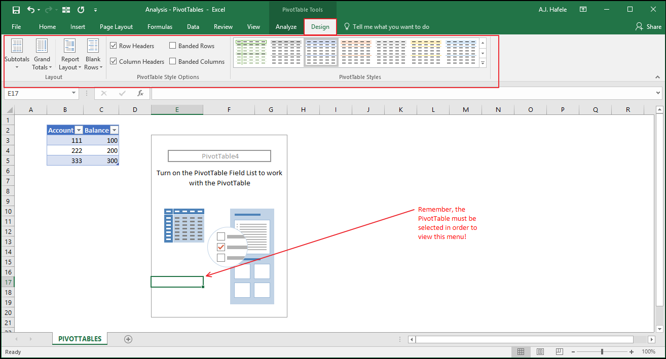
Additionally, two new menus are available when a PivotTable is selected
The first one is the Analyze tab:
The second one is the Design tab:
There are also a few more menus (particularly the PivotTable Options and Field Settings menus) that we will cover in the below discussion
This Lecture's Example
Imagine you are a company with 4 products: Products A, B, C and D
You sell the products in 4 regions: North, East, South and West
You want to analyze both revenues and expenses relating to each product
You want to examine historic trends in these variables from 2021 to 2030 (imagine the current year is 2031)
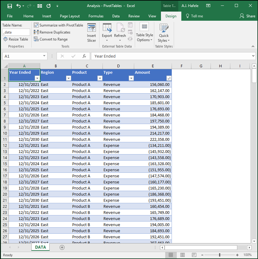
We have compiled a table containing this data (in the DATA tab of this lecture's Excel file)
This data will be used to illustrate how PivotTables work in the sections below
Organizing Raw Data
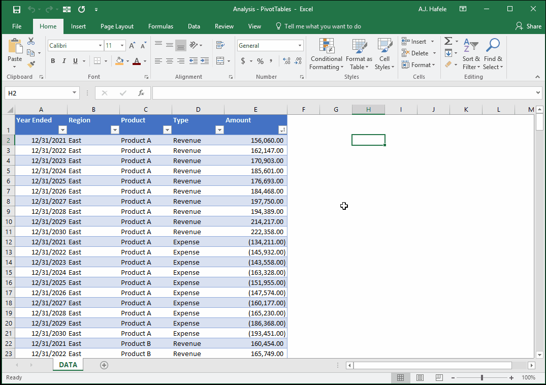
First and foremost, it is absolutely critical that your underlying data be organized in a tabular format, and ideally in a table (as we will use in this lecture)
This is necessary in order to extract the most value out of your PivotTables
In particular, having data in a tabular format will allow you to optimize your PivotTables' flexibility
Here is a screenshot of our table, for reference:
Importantly, note that the table's name is "_data", as shown in the top-left corner of the above screenshot (in the Design tab)
Also note that revenues are positive Amounts, and expenses are negative Amounts
Insert a PivotTable
To insert a PivotTable into a worksheet, move the active cell to any cell in your table, and click the PivotTable button from the Insert tab (or use the ALT, N, V shortcut)
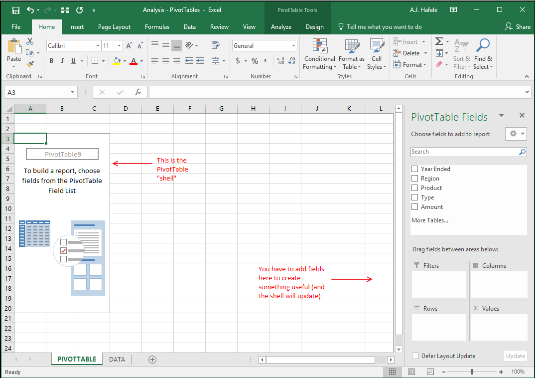
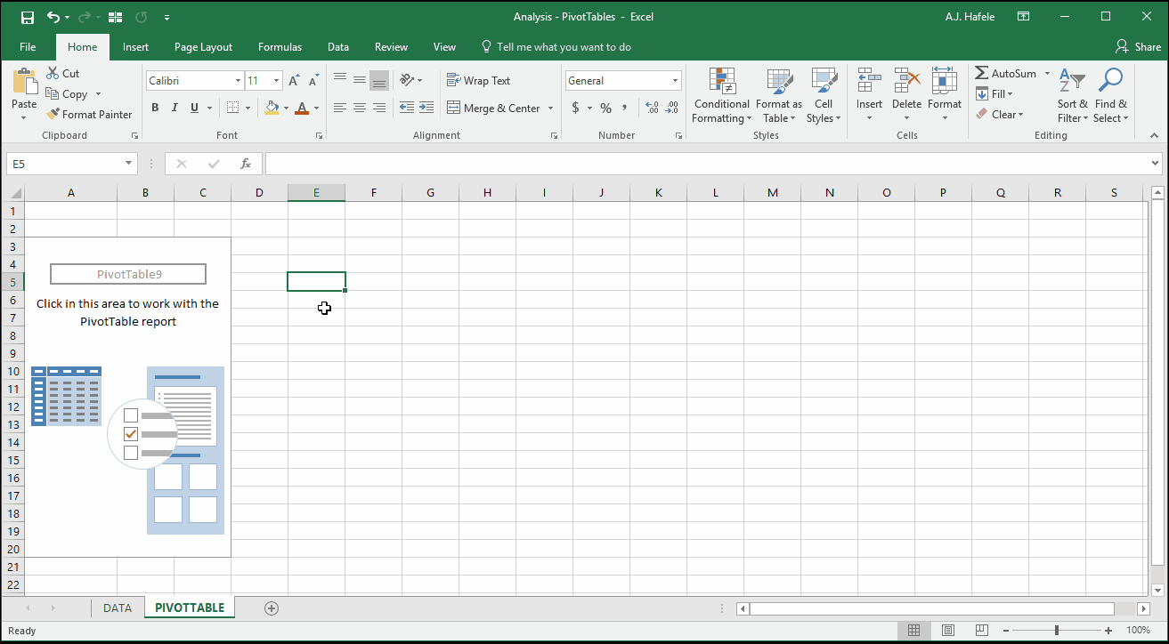
Let's create a PivotTable and place it in a new worksheet called "PIVOTTABLE":
Here is a screenshot of the resulting PivotTable:
Note that the above PivotTable is effectively a shell, as no fields have been added as rows, columns, filters, or values (per the bottom-right side of the screenshot)
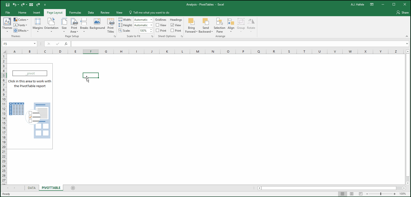
As an alternative to placing your PivotTable in a new worksheet, you may want to place the PivotTable in an existing sheet, as shown here:
We highly recommend placing PivotTables in their own worksheets in order to avoid overlap between PivotTable, and non-PivotTable data
PivotTables, when updated / refreshed, can actually overwrite non-PivotTable data
Last, let's quickly rename the PivotTable "_pivot":
Add Rows, Columns, Values and Filters
Thus far, all we have is a PivotTable "shell" that is not very useful, so let's change that by adding rows, columns, values and filters
But first, always remember to keep in mind your objective / question when creating PivotTables
Let's define a few objectives and build the appropriate PivotTable for each
Importantly, there are multiple ways to achieve the same objective!
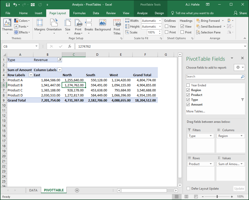
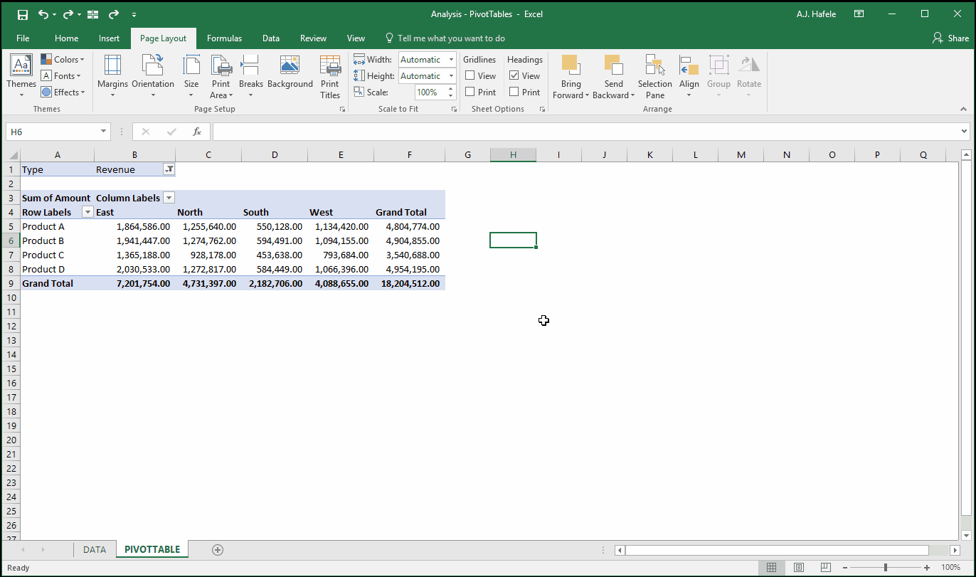
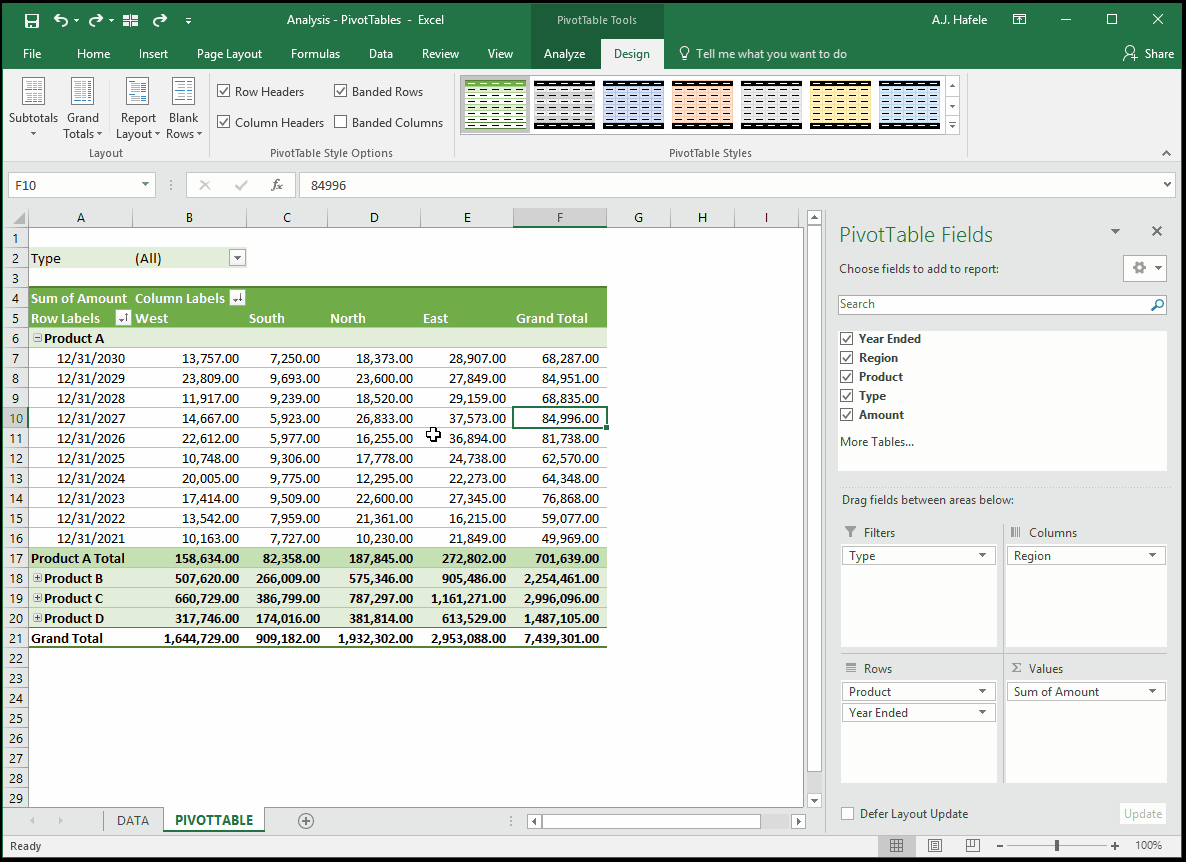
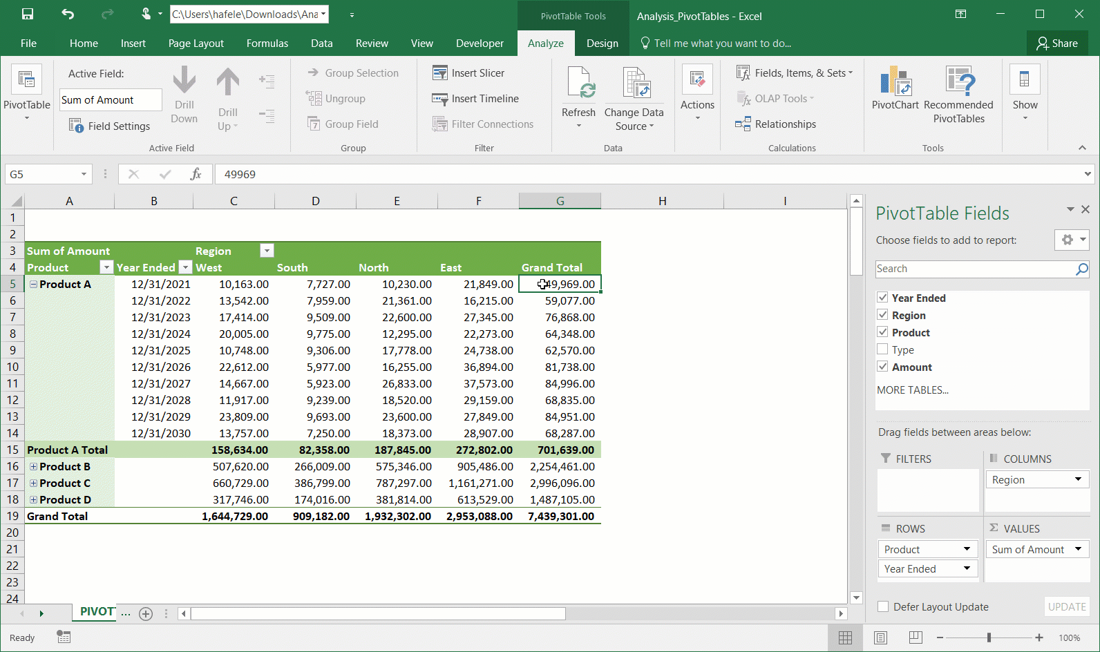
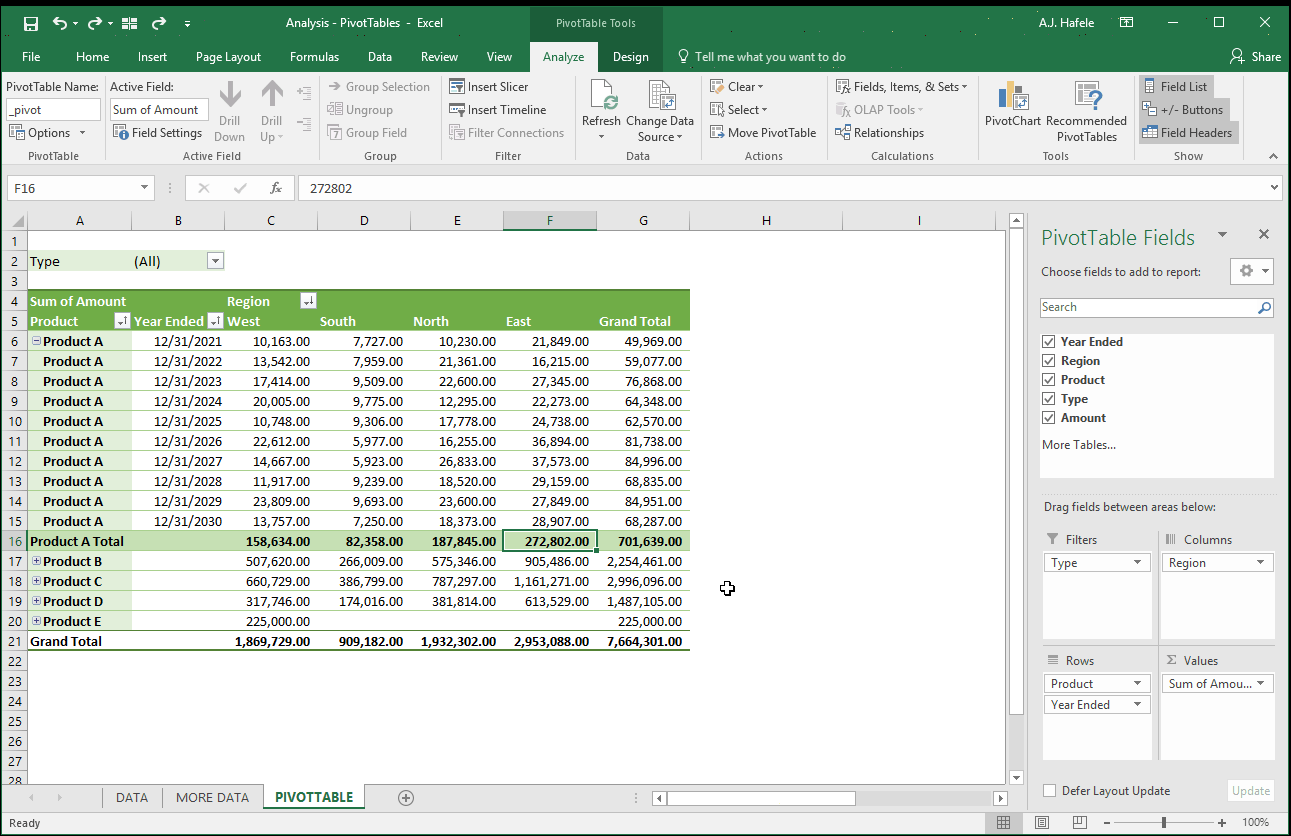
Objective 1: Determine total 10-year revenue by region and product:
Notice that all we needed to do was click and drag the fields! (well, we also did some formatting of the values in the above illustration)
Screenshot of result:
Since we wanted to view total revenue summed across all 10 years, notice that we completely excluded the Year Ended field from the PivotTable
Interpreting this PivotTable:
Product B revenues in the North region from 2021 to 2030 were 1,274,762
Total Product A revenues from 2021 to 2030 were 4,804,774
Total East region revenues from 2021 to 2030 were 7,201,754
Total revenues for all products and regions from 2021 to 2030 were 18,204,512
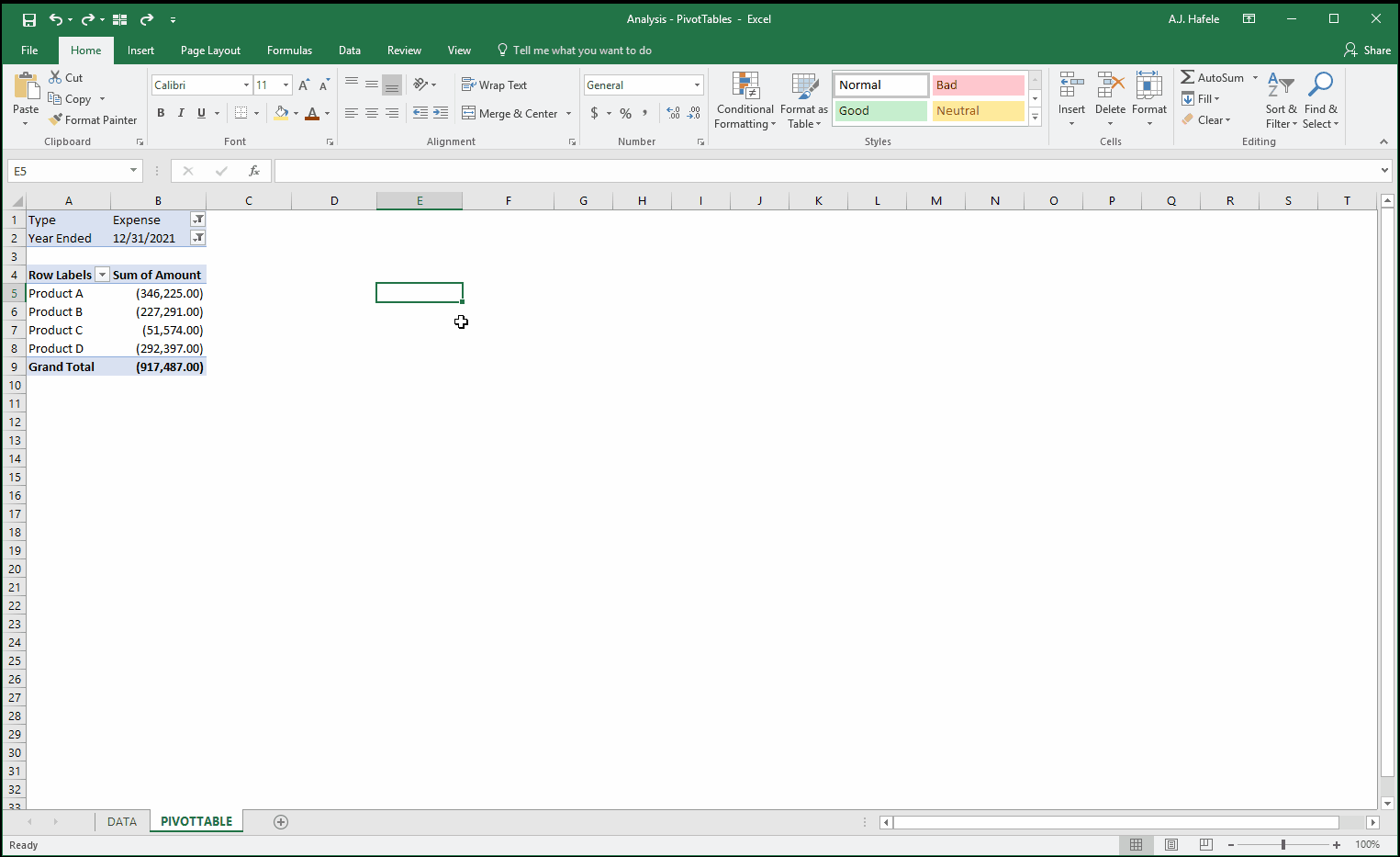
Objective 2: Determine total expenses by product in 2021:
Screenshot of result:
Note the following
This time, we did not need any column of data, since we care only about the Product field (the rows)
We did not need to break out the expenses by region this time
However, we now have 2 filters instead of 1
The first is to filter for expenses only
The second is to filter for the year 2021 only
Interpreting the PivotTable:
Total Product A expenses across all regions in 2021 were 346,225
Total expenses across all regions in 2021 were 917,487
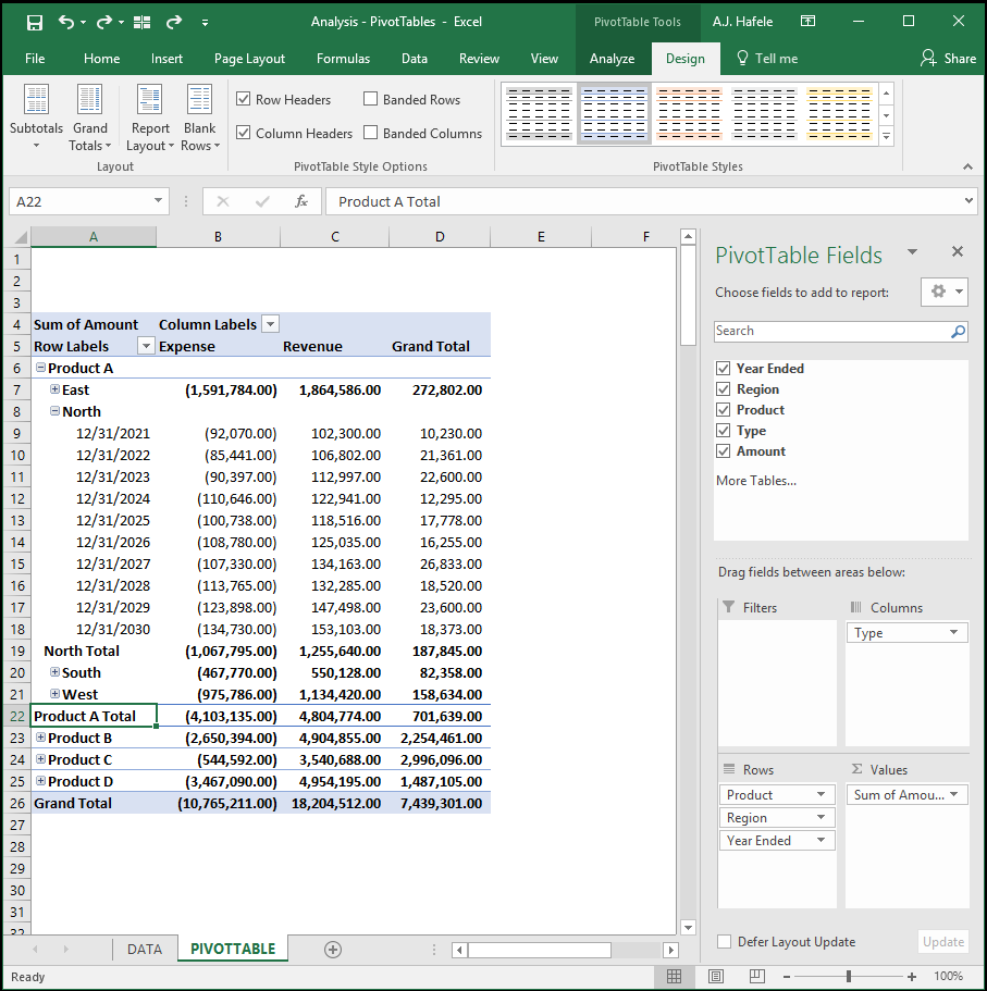
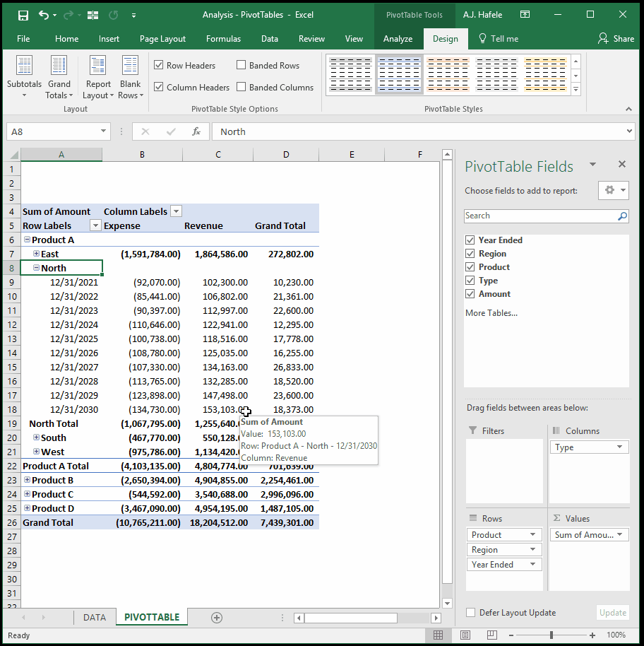
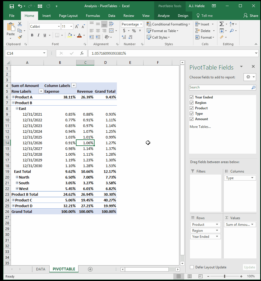
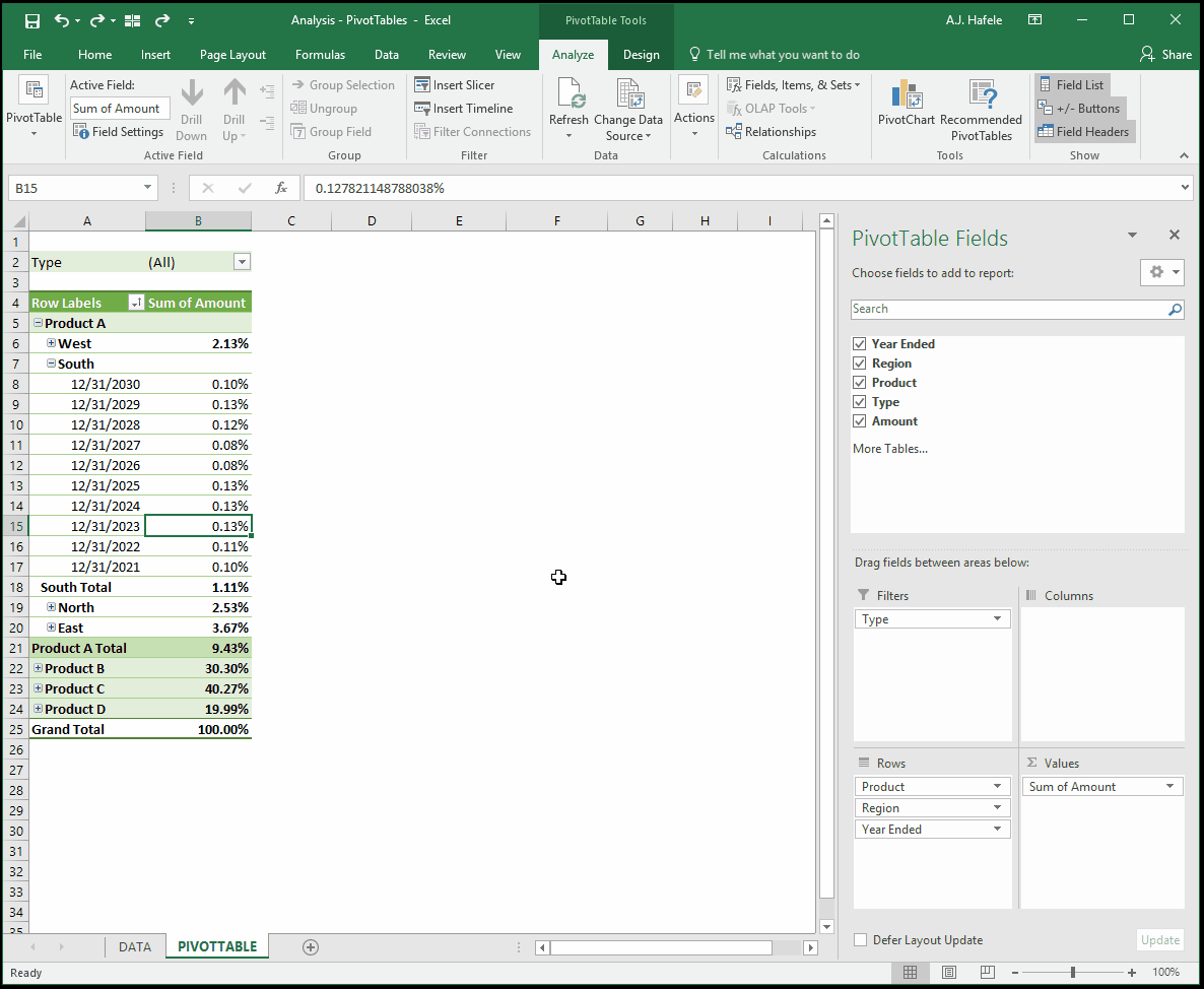
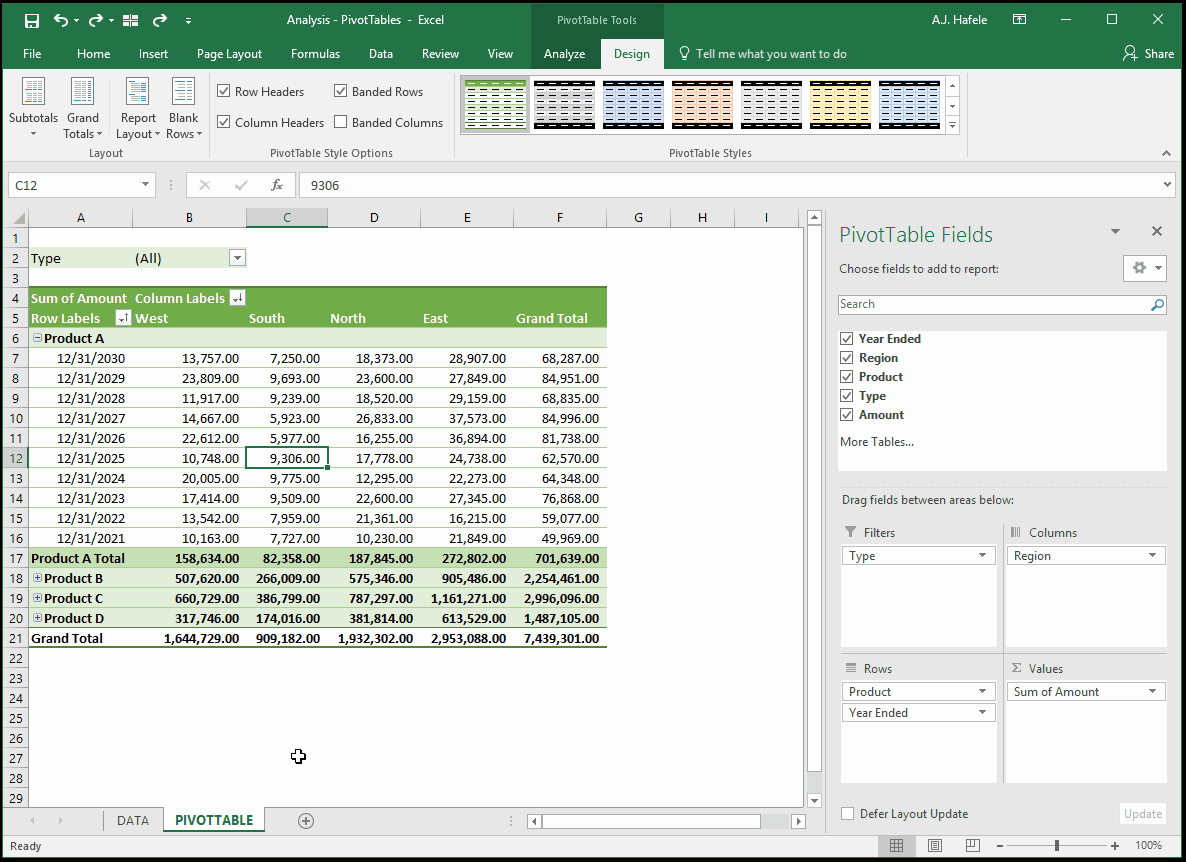
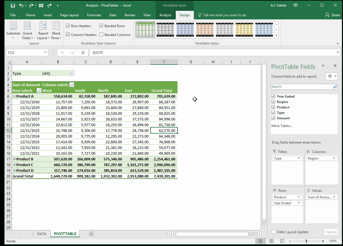
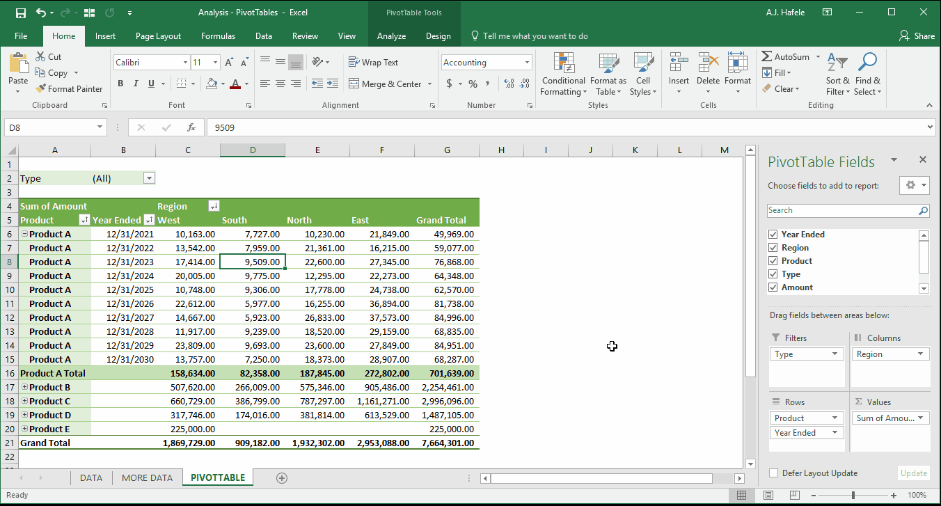
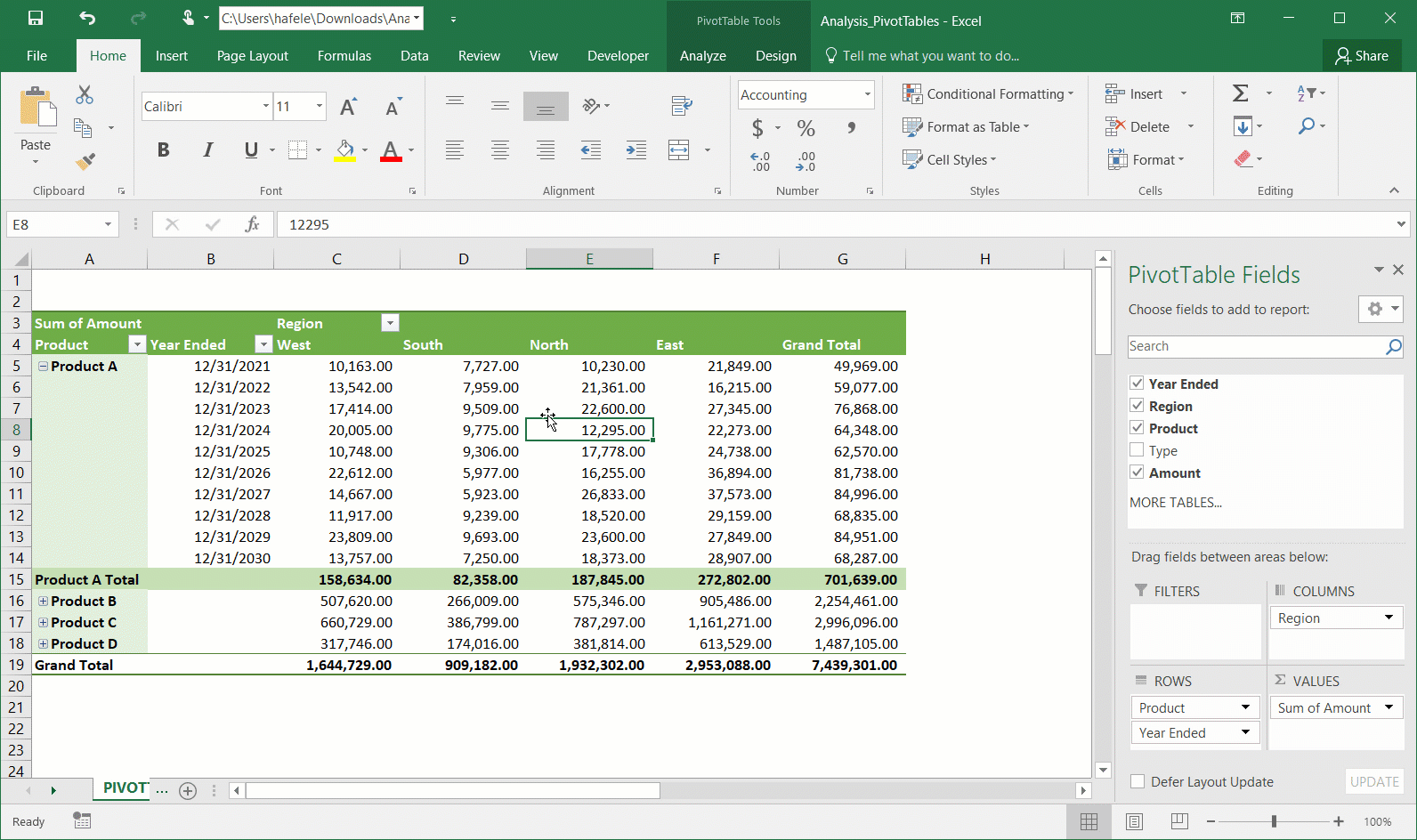
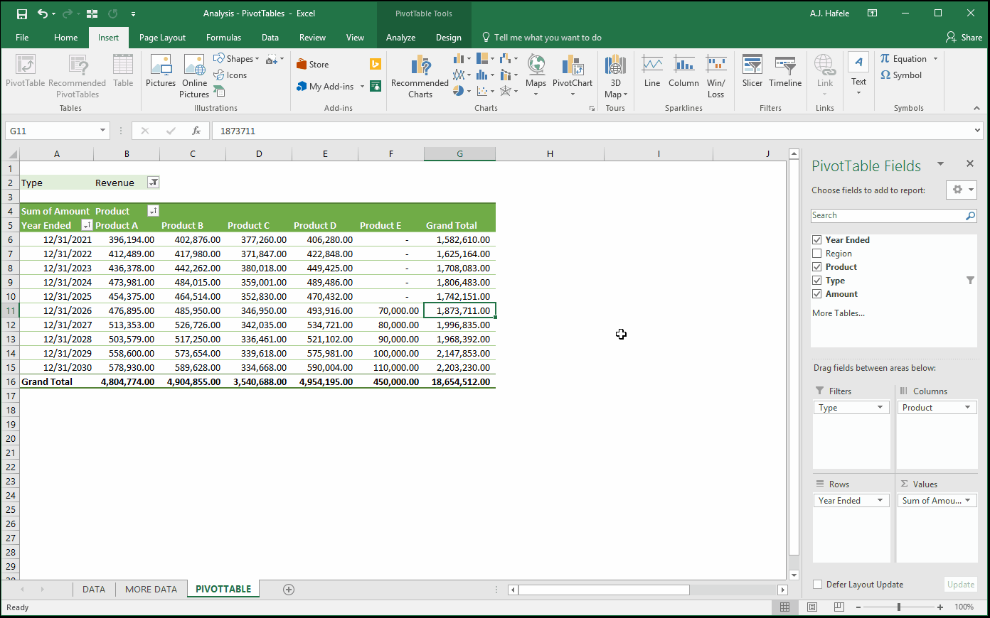
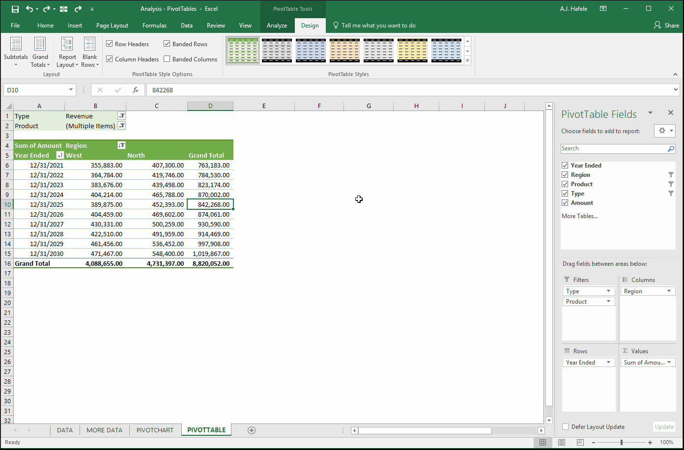
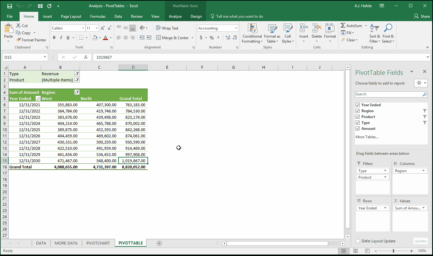
Objective 3: Determine revenues, expenses, and net revenues by product, region, and year:
Screenshot of result:
Note the following:
We now have 3 fields as rows - Product, Region and Year Ended. Notice that we can collapse/expand the fields to drill down to the relevant level of detail (as shown with Product A in the North region in the screenshot)
We now have 1 field as the column, which shows us total expenses, revenues, and net revenues (the Grand Total column) for each row
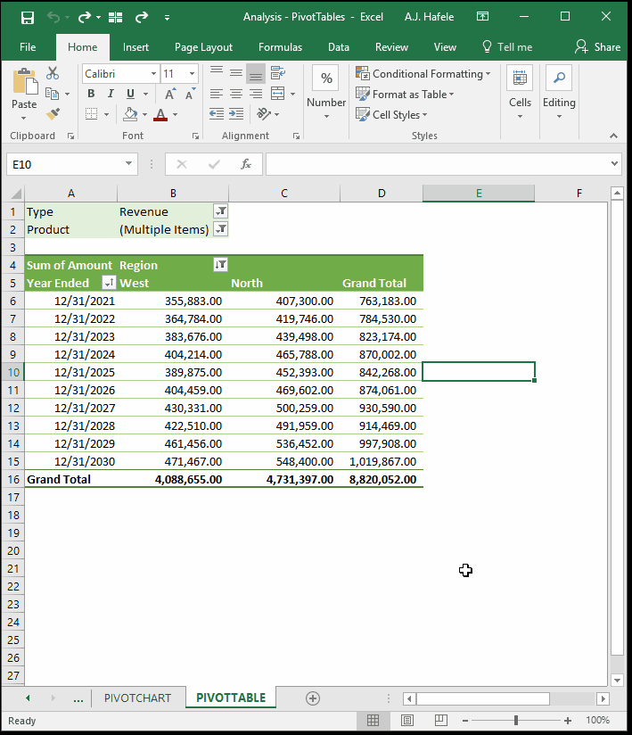
Interpreting the PivotTable:
Product A revenues in the North region in 2021 were 102,300
Total Product A revenues in the South were 550,128 over the 10-year period
Total Product B expenses -2,650,394
Total net revenues across all products and regions were 7,439,301
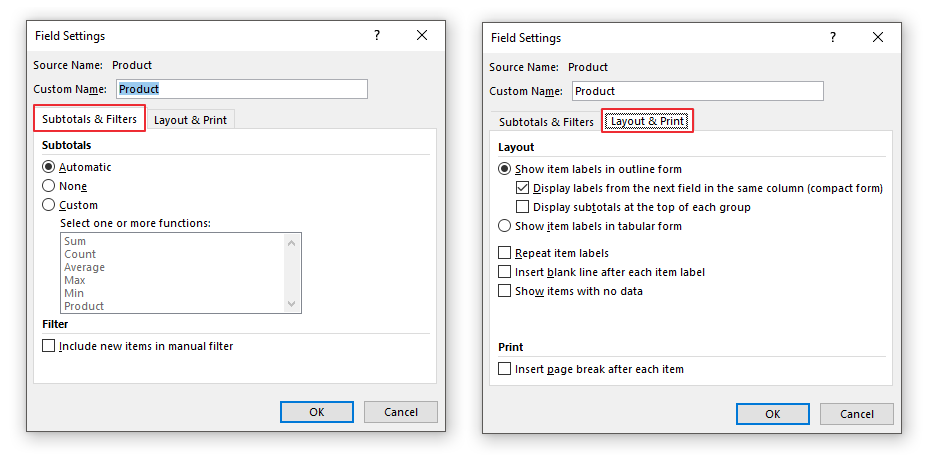
PivotTable Field Settings
You may have noticed in the Objective 1 example above that we changed the format of the values to Accounting (without the $ symbol) for better readability. This change was made in the one of the Field Settings menus
Let's look more closely at these settings to see what we can modify
There are actually two different PivotTable Field Settings menus
The first menu - Field Settings - is used for rows, columns, and filters:
These options are self-explanatory: the first tab allows you to specify the subtotals performed (if any), and the second tab allows you to change the field's layout
Note that there are buttons in the Ribbon that perform the same function, so we will discuss these in the sections below
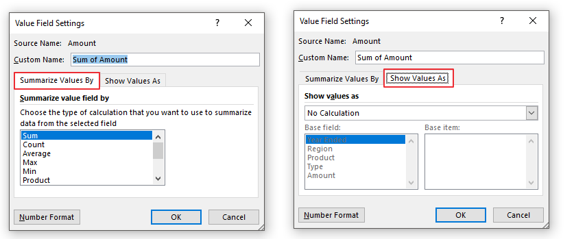
The second menu - Field Value Settings - is used for values:
The first tab allows you to choose the PivotTable calculation being performed
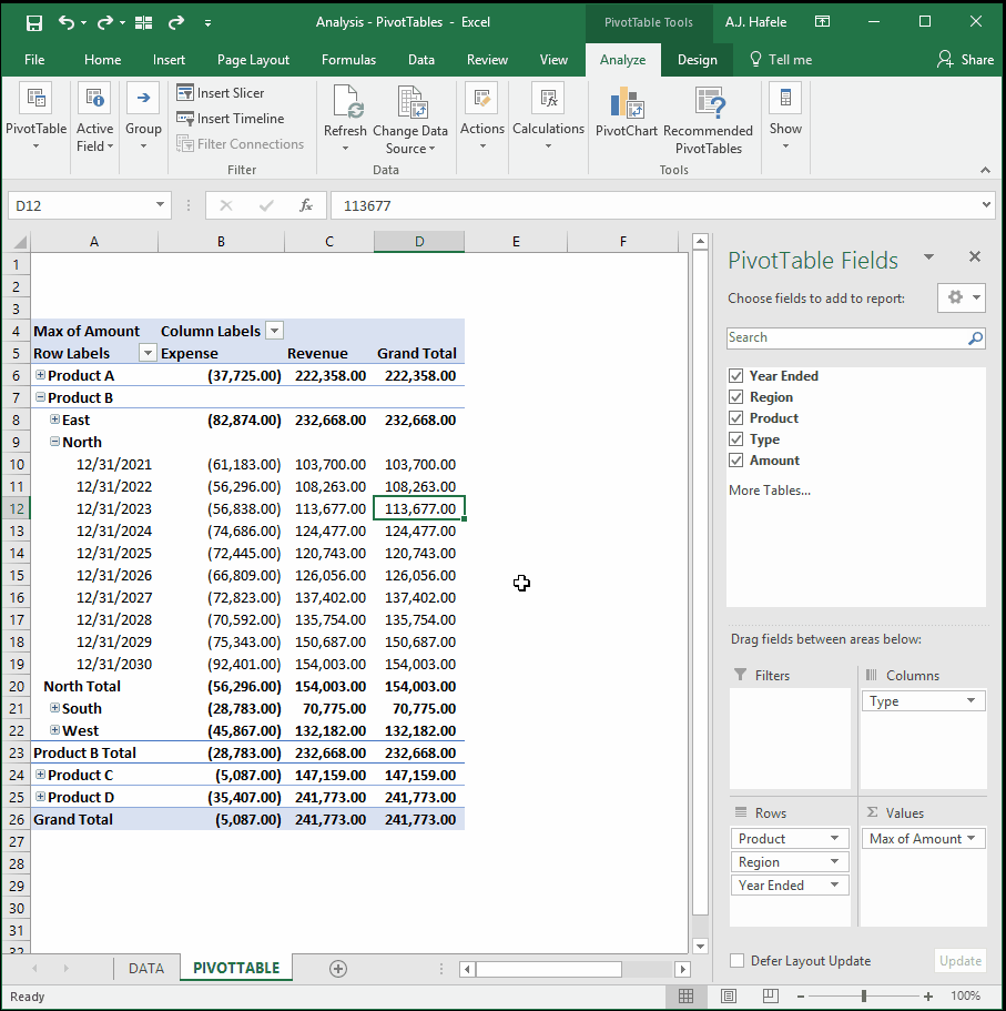
Instead of computing the sum, let's compute the max (maximum values):
The PivotTable works in the same manner as sum, except the max (the lowest expense, and the highest revenue) is being calculated instead
The max will dynamically adjust when expanding/collapsing fields
The second tab (the Show Values As tab) allows you even greater flexibility in presenting the fields
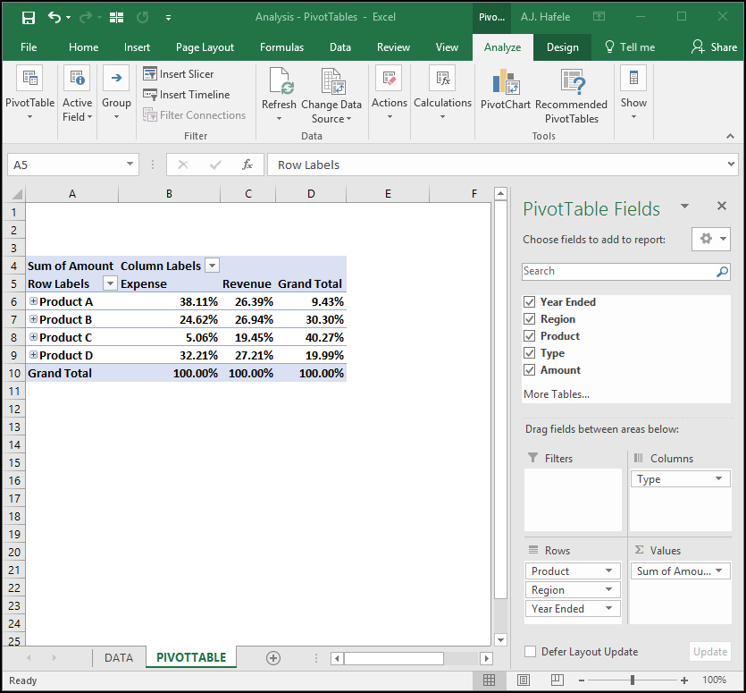
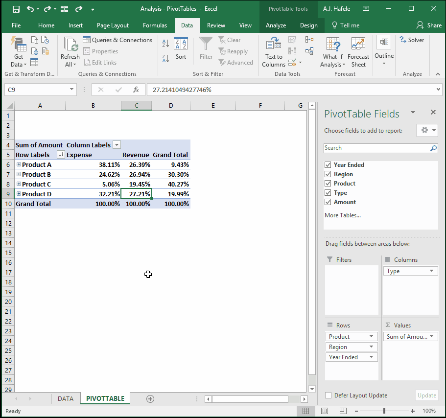
For example, what if we wanted to present the totals (using sum, not max) as a percentage of total expenses, revenues, and net revenues? Observe:
Screenshot of result:
The PivotTable clearly indicates that, while Product C's total revenues were the lowest (19.45% of the total), it's net revenues were the highest (40.27% of the total) since its expenses were the lowest (5.06%)
Last, if you re-examine the Field Settings menus, you will notice that you also have the ability to rename the fields
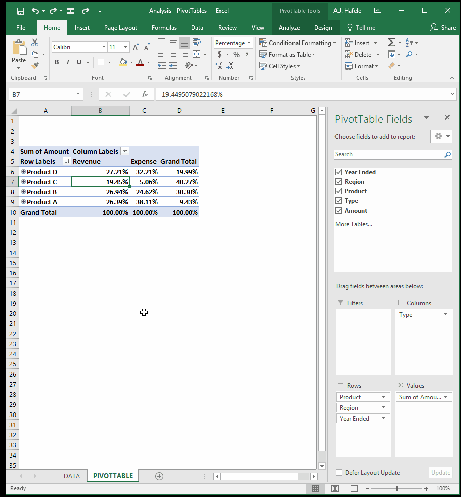
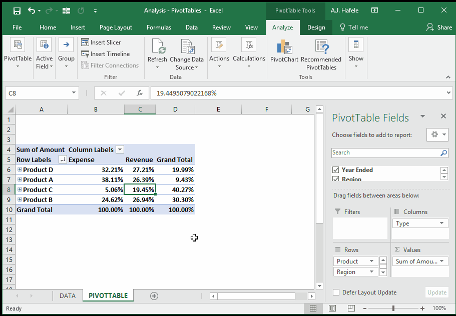
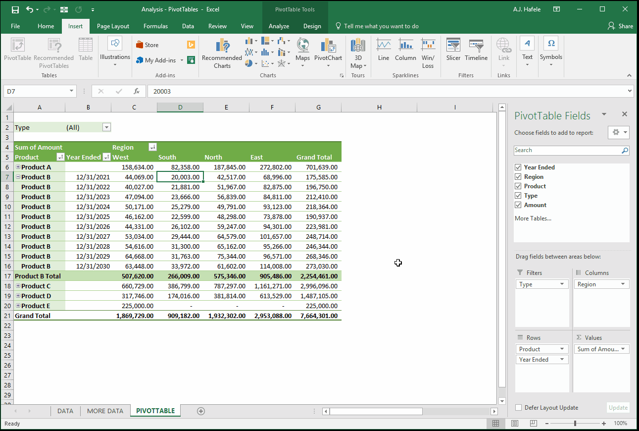
Sort PivotTables
There are a number of ways to sort PivotTables
The first way is to use the filter buttons within the PivotTable, as shown here:
The second way is to manually type the data in the rows and columns (in any order you wish):
A third alternative to sort the rows is to utilize the buttons in the Data tab, as shown here:
Filter PivotTables
There are a number of ways to filter PivotTables
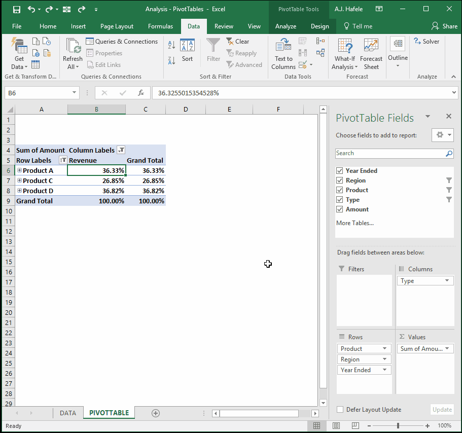
First, the filter buttons within the PivotTables can be used, as shown here:
Alternatively, if a field is not needed as a row or column, it can be placed exclusively as a filter in the PivotTable
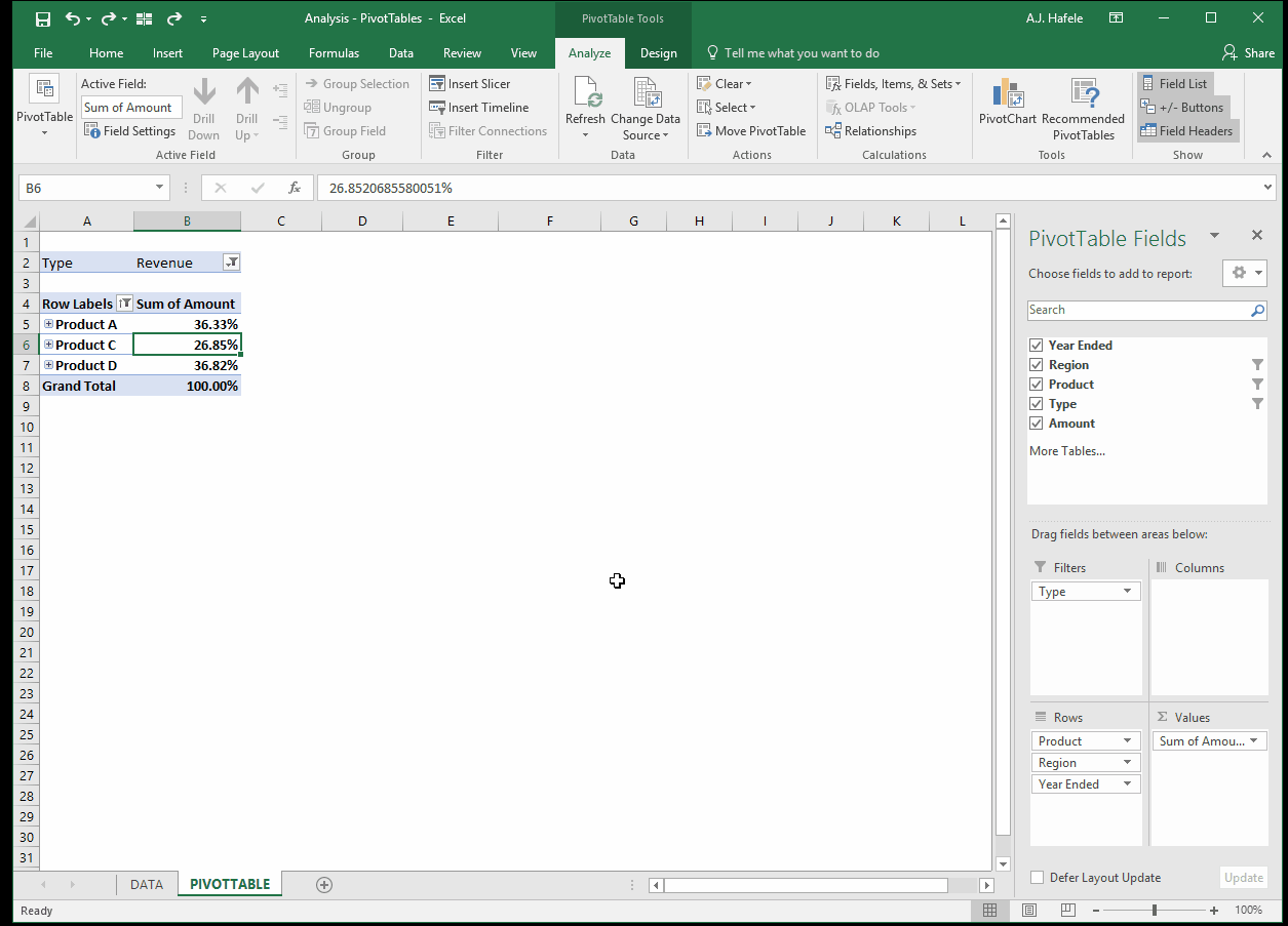
In the previous illustration, notice that the Grand Total was no longer necessary after filtering for revenues only; we could just move the Type to the filter bucket instead, as shown here:
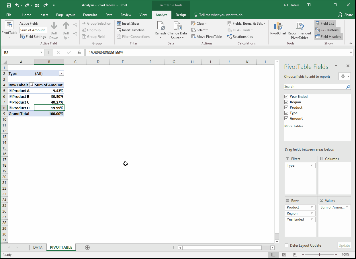
Last, let's clear all filters:
As a side note, you can also use the Clear Filters button located in the Data group of the Analyze tab
Grouping Rows and Columns
In addition to sorting, filtering, and rearranging data, Excel enables you to specify groups of data
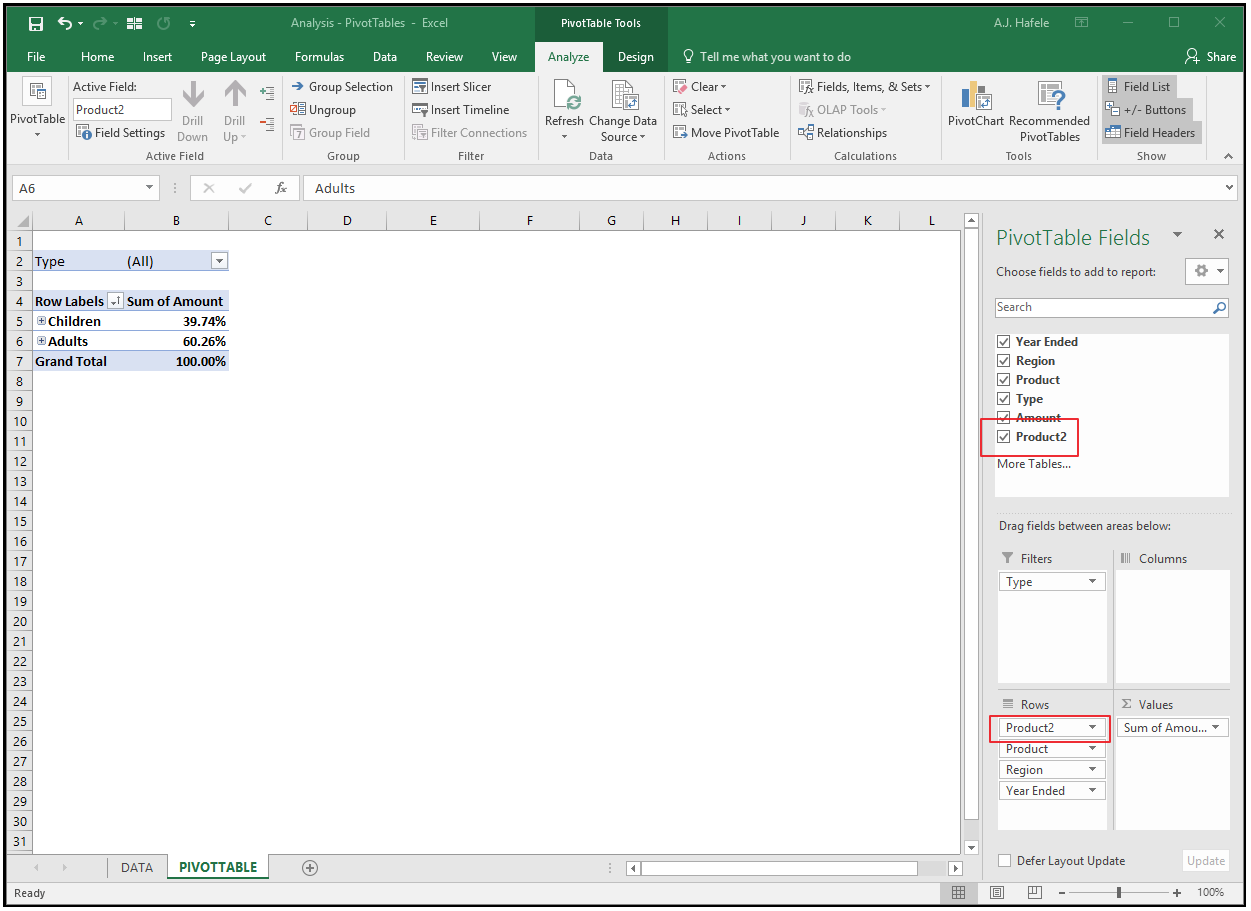
Imagine that Products A and B are for children, and Products C and D are for adults. We can group them as such, as follows:
Notice in the below screenshot that Excel automatically created a new field called Product2, giving all line items corresponding to Products A and B a value of "Children" (and similarly, giving a value of "Adults" to Products C and D):
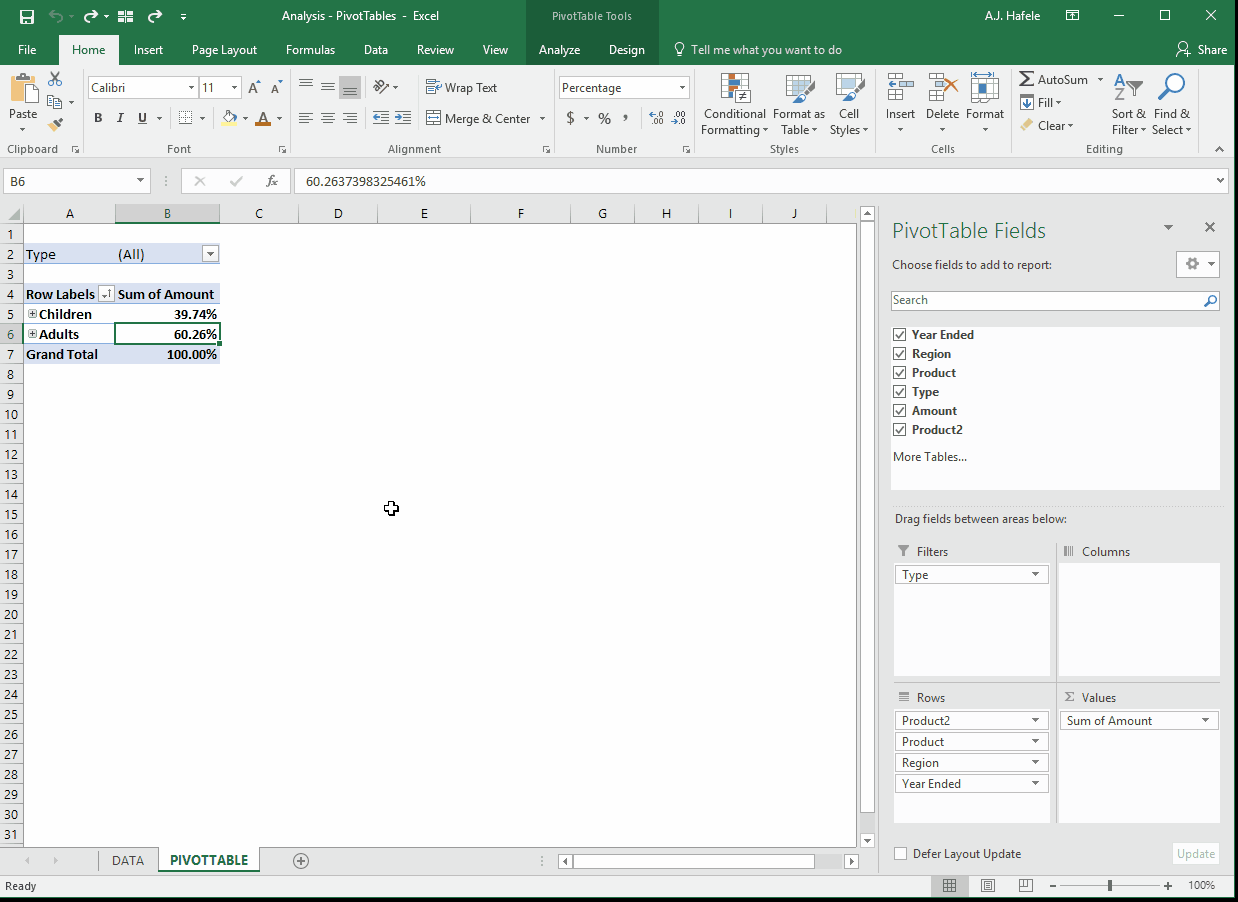
Remember that this field can be renamed in the Field Settings menu, as shown here:
Although not shown in our illustrations, columns can be grouped in the same manner
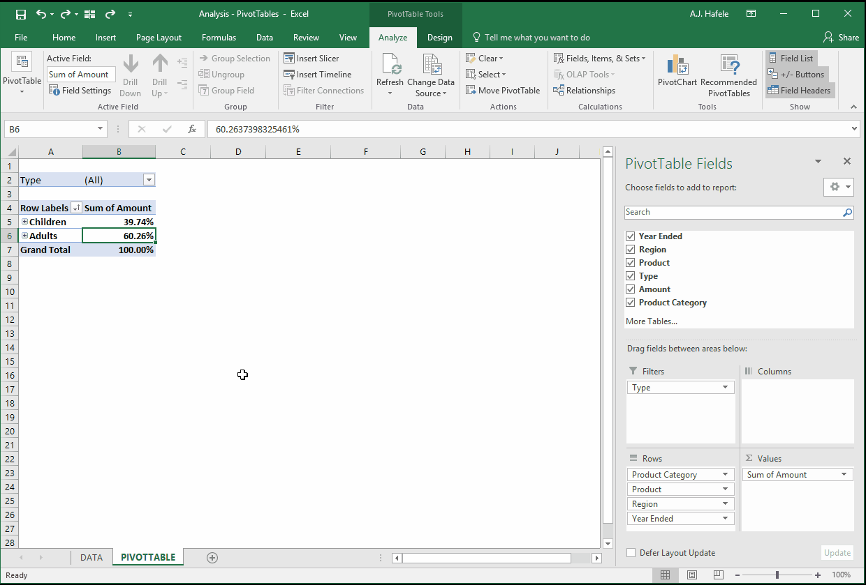
Now, let's illustrate how to ungroup:
Notice in the above example that the "Product Category" field (in the Rows section) goes away after the ungroup
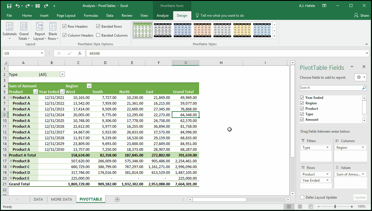
PivotTable Styles
In many instances, you will be sharing your PivotTables with others, so you will want to make sure it is easy to read / comprehend
Excel has many pre-defined PivotTable styles which can be used to enhance the clarity of the data
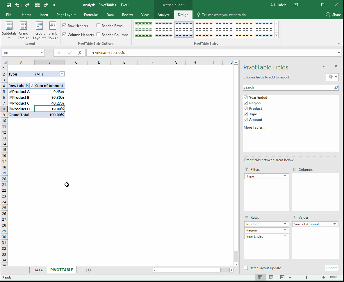
In the following illustration, the PivotTable is already pretty easy to understand, but we will modify the PivotTable style to show you some of the options that are available:
Although the new (green) style is not extremely different, it does have the added benefit of color-coding some of the row groupings in various shades of green
Nevertheless, you may encounter instances in which changing the style can drastically improve the clarity of your data
PivotTable Layout Options
Let's now see what the Layout options (in the Design tab) can do
But before we get into some examples, let's present the Region field as columns, and let's change the Values to present net revenue amounts (not percentages):
Observe as subtotals and grand totals can be modified:
We can also add blank rows between items, as shown here:
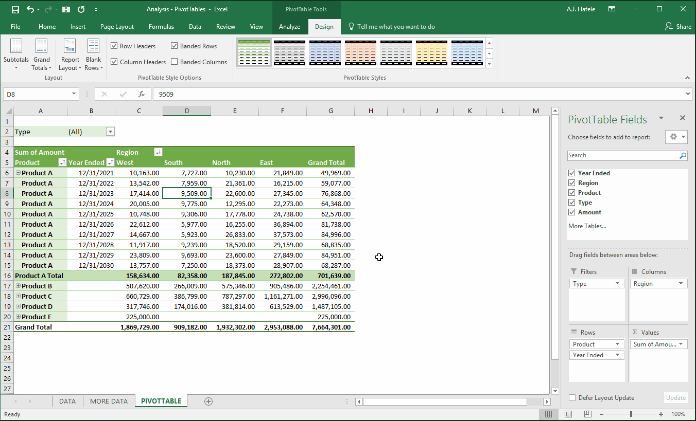
Last, you have a number of options allowing you to change the report layout, as shown here (note that we start with Compact Form):
One nice aspect of using Outline Form or Tabular Form is that the Year Ended field is now in its own column (so we can sort directly from that column)
This is particularly useful when you have many fields placed as rows
Refresh PivotTables
Remember that PivotTables present summaries (and other views) of underlying data
In our example, the underlying data is the information contained in the _data table (in the DATA sheet)
If your PivotTable's source data is modified (i.e. data are added or removed, or changed), the PivotTable will not reflect the change until it is refreshed!
Therefore, if your source data changes, be sure to refresh your PivotTables regularly, or your analyses may be inaccurate!
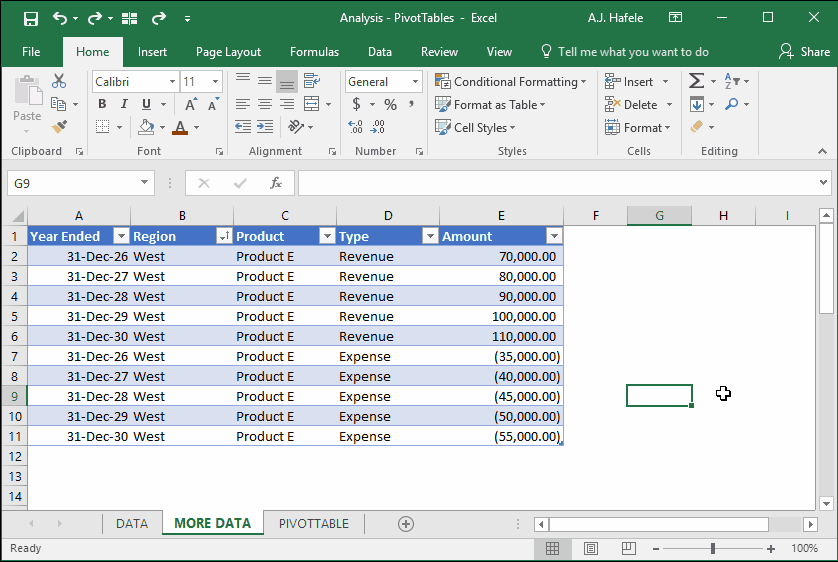
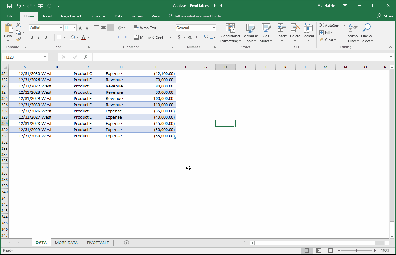
To illustrate the importance of refreshing PivotTables, let's add data for a new product - Product E - to the _data table:
Continuing our example, let's look at the PivotTable before and after we refresh:
Note that:
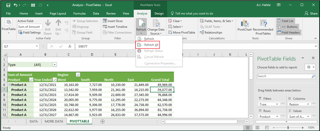
Before the refresh, Product E did not exist in the PivotTable (even though it was in the underlying table!)
After we clicked Refresh, Product E appeared in the PivotTable!
Remember that Product E was only sold in the West - that is why you see blank data for the other regions
Though not shown above, you can also use the ALT+F5 or ALT, J, T, F, R shortcuts to quickly refresh any selected PivotTable
As a side note, if you are working with multiple PivotTables and want to refresh them all simultaneously, simply click the Refresh All button in the Analyze tab,(ALT, J, T, F, A) as shown in the following screenshot:
In addition, Excel gives us the option to automatically refresh PivotTables each time the file is opened (via the PivotTable Options menu)
To choose this option, do the following:
Note that when this option is selected (or deselected) on a given PivotTable, the option is also selected (or deselected) for all PivotTables linking to the same data source
In our example, all PivotTables linking the _data table will now refresh when we open the Excel file
Change PivotTable Data Source
To change a PivotTable's data source, simply click the Change Data Source button in the Analyze tab, as shown here (changing the source from the _data table to the data_2 table):
Note that we clicked Undo in the above example to revert back to using the _data table as our data source
Once again, the major advantage of using tables when creating PivotTables is that you do not have to worry about re-selecting your data source once data are added to (or removed from) your table
Calculated Fields
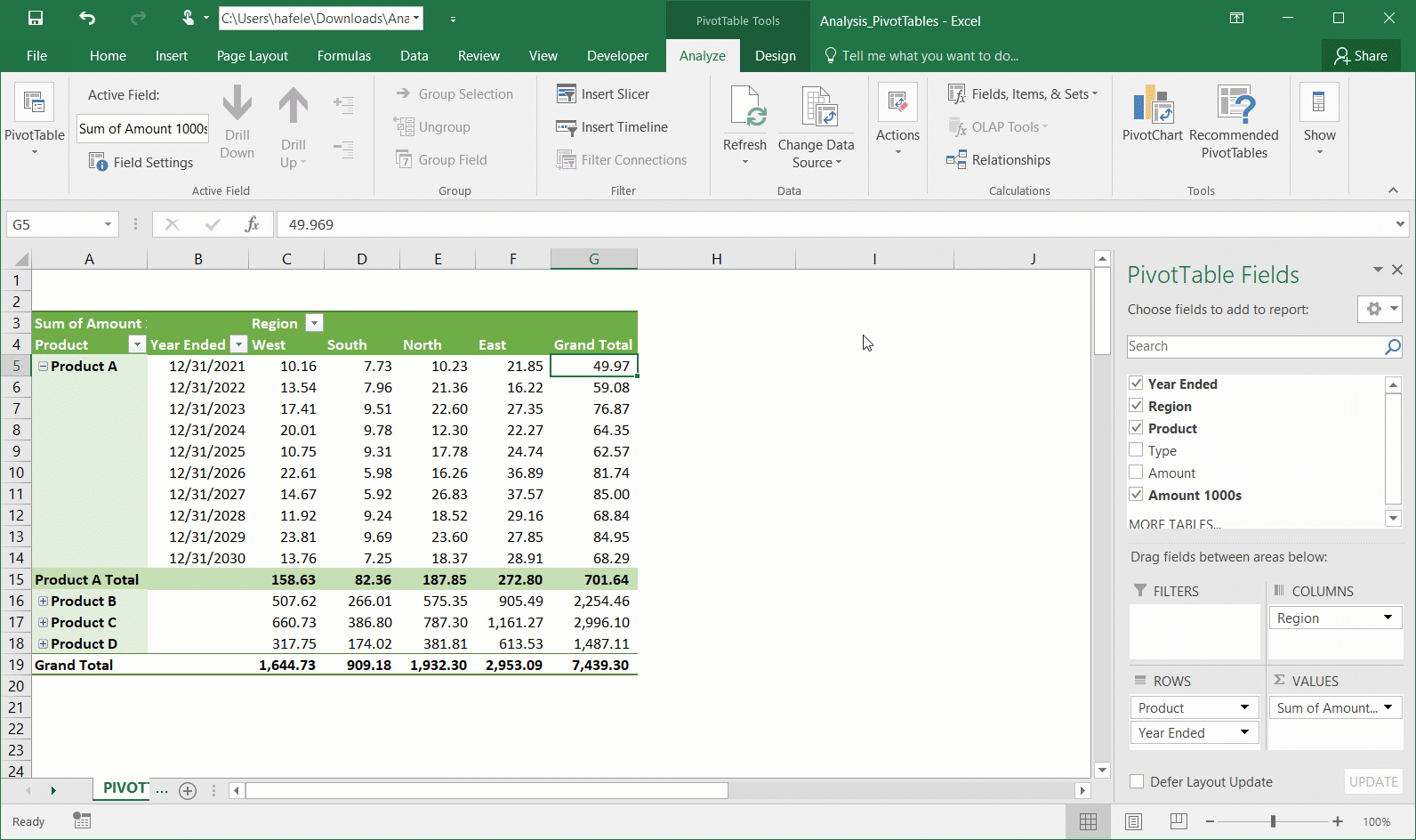
Imagine we want to present our PivotTable amounts in thousands of dollars, rather than dollars
We can create a calculated field that divides the Amount field by 1,000, as shown here:
This was a pretty simple example, but of course more complicated calculated fields can be created
Also note that, instead of creating a calculated field, a new field (with the same calculation) could be added to the underlying table
The following illustration shows how to delete a calculated field (we also re-add and format the Amount field):
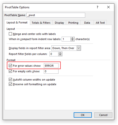
Replacing Blank Values and Error Values
Let's quickly review a few useful PivotTable formatting options
First, sometimes you may want to replace blank values in a PivotTable with another value
That can be done as shown here (zeros will be shown as dashes):
Note that the same can be done for error values here (screenshot):
Autofit PivotTable Column Widths
By default, PivotTable columns will Autofit upon refresh (i.e. they will change widths based on the contents of the PivotTable)
Observe how Autofit works, and how we can stop it:
Adding and Removing Expand / Collapse Buttons
You may have noticed that some of the rows in our previous examples have +/- (expand/collapse buttons) in the leftmost columns
To remove these buttons (and to re-add them), do the following:
Remember that you can still expand/collapse the data by double-clicking the relevant fields (as shown above), so this is primarily a cosmetic change
PivotCharts
Sometimes, a chart of a PivotTable can be more revealing than the PivotTable itself
In that case, PivotCharts can be very useful
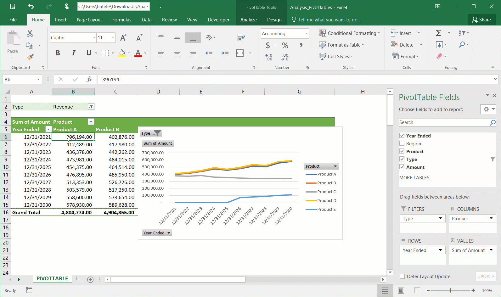
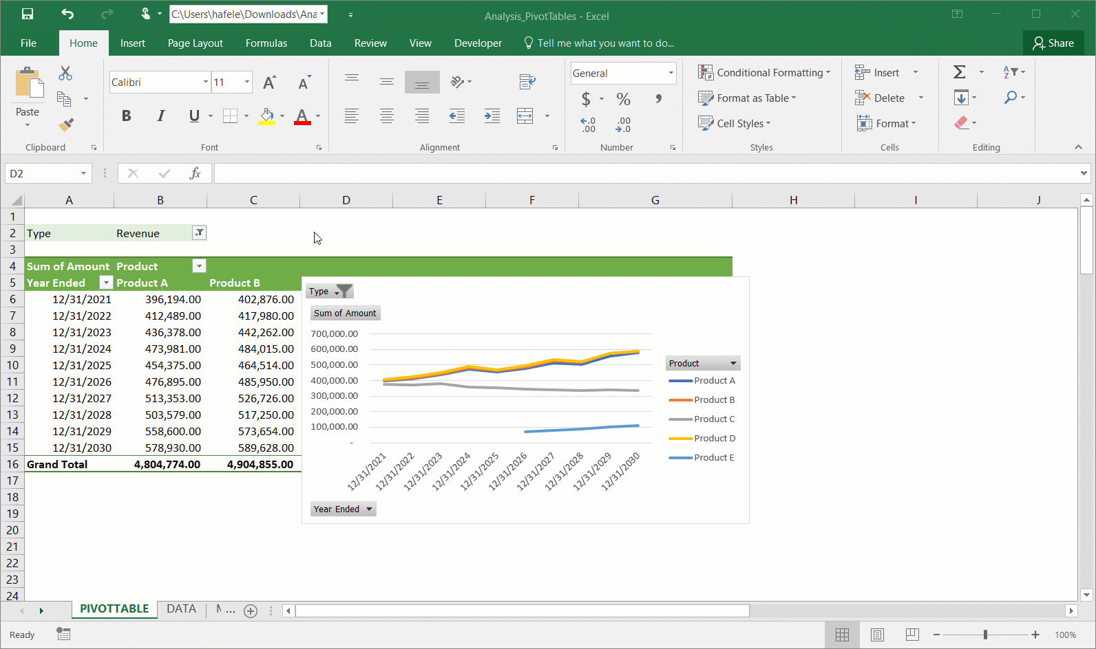
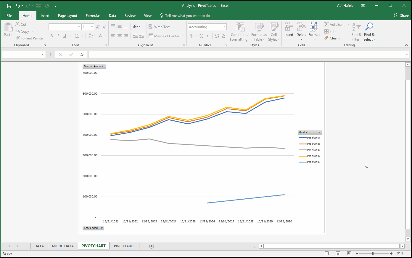
Let's demonstrate by plotting revenue by product over time (via a line chart)
First, let's adjust the PivotTable:
Now let's create the PivotChart (shortcut is ALT, N, S, Z, C):
Now let's replace blank values with nothing (not "0") so we do not chart 0 values (keep an eye out on the Product E line in the chart); let's also move the chart to a new sheet:
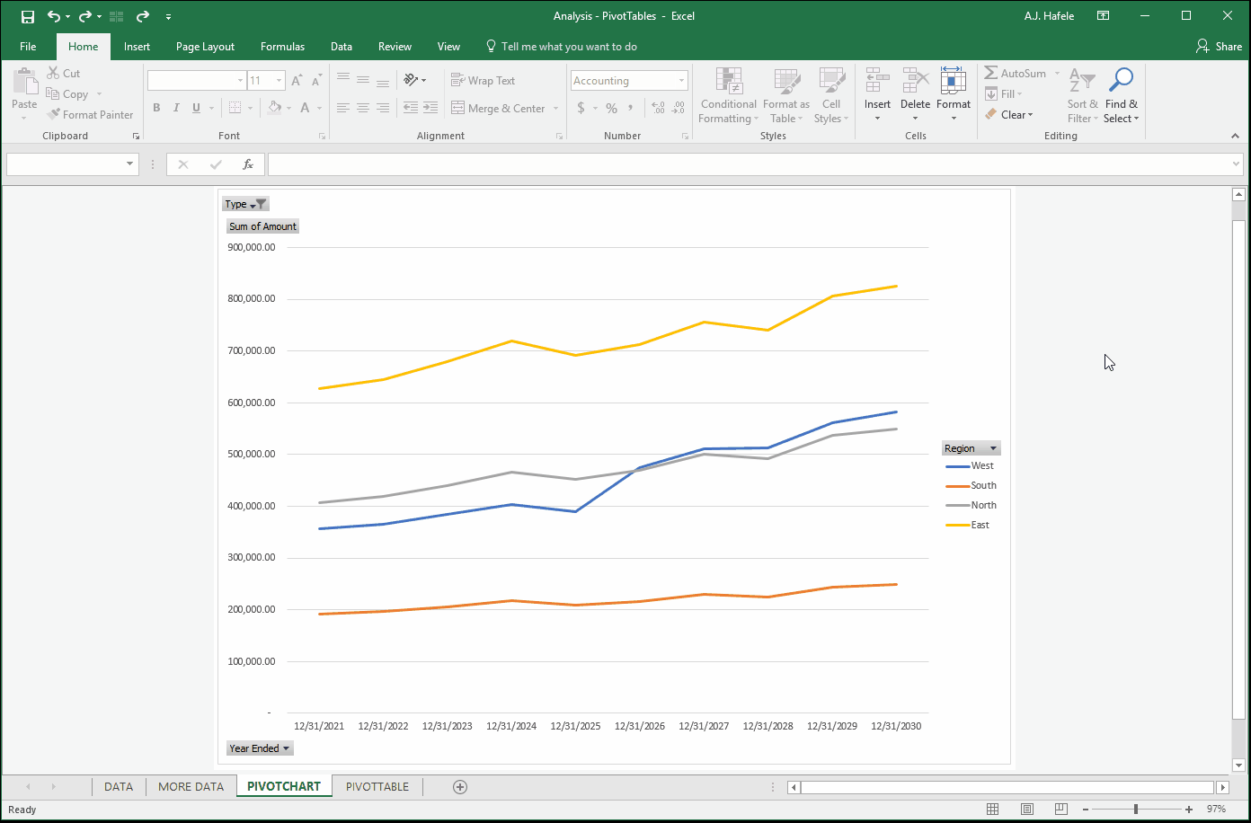
Now let's chart revenues by region instead:
Note that if you need to create multiple PivotCharts, you may need to create multiple PivotTables (if those PivotCharts require a differently-structured PivotTable)
Last, let's filter out Product E (since it is only sold in the West region) from the PivotChart, and compare revenues from the West and North only:
Note that we also cover PivotCharts briefly in the charts lecture
Move PivotTable
Excel enables us to move PivotTables within an existing sheet, or within a new sheet
Let's illustrate how to move a PivotTable within an existing sheet (we will Undo after we move):
Tracing PivotTable Values (To Source Data)
Sometimes you may need to figure out how a PivotTable computed a certain value
This is easily done by double-clicking any value in the PivotTable, as shown here:
As you can see, double-clicking the value places a table of data in a new sheet
The figures in this new (scrap) table are derived from our source data table (_data, in our example)
Think of this data as an excerpt of the underlying source data
This is extremely useful when you need to audit numbers
Delete PivotTables
To delete a PivotTable, simply select it (all of it) and press the DELETE button
Alternatively, you can delete all the rows and columns it encompasses, as shown here:
Organizing Your Data - Use Tables
To reiterate, PivotTables are best used when the underlying data are stored in tables
Why? Because when data are added or removed from the table, the PivotTable will dynamically adjust to those changes
The value of placing your source data in a table cannot be understated! Always use tables!
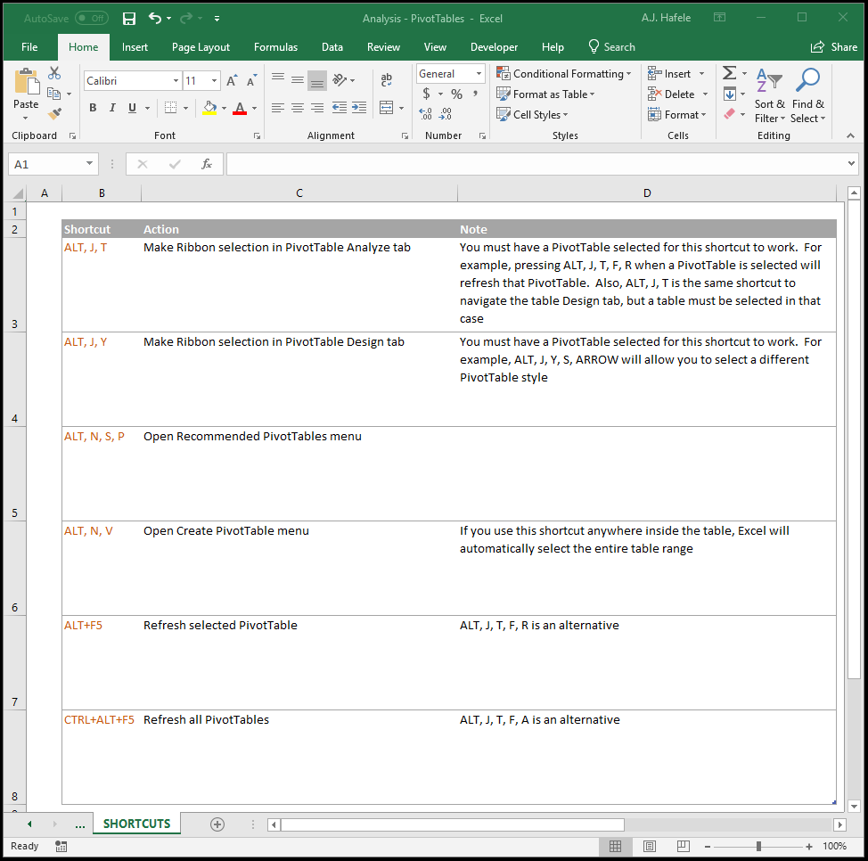
Shortcuts
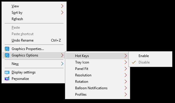
If the CTRL+ALT+F5 shortcut is not working properly, try disabling Hot Keys by right-clicking your desktop and choosing Disable in the following menu: